|
|
|
Spatial
Convolution (Blurring)
Example 1
Create an
average filter and move it over an image. Display the new
image.
Solution
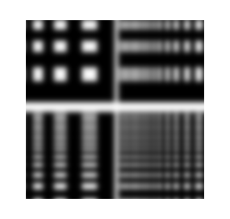
im = imread( 'testpat2.tif');
imshow(im)
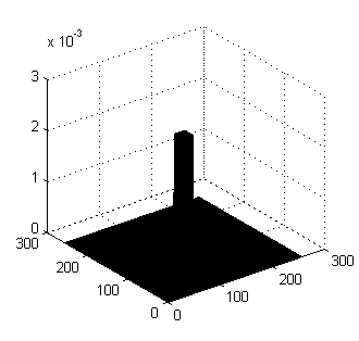
avfilter =
fspecial('average',[21
21]);
figure, surf(avfilter);
newim=filter2(avfilter,im);
figure,
imagesc(newim);
Result

Spatial
Convolution (Blurring)
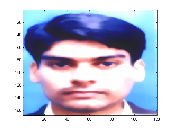
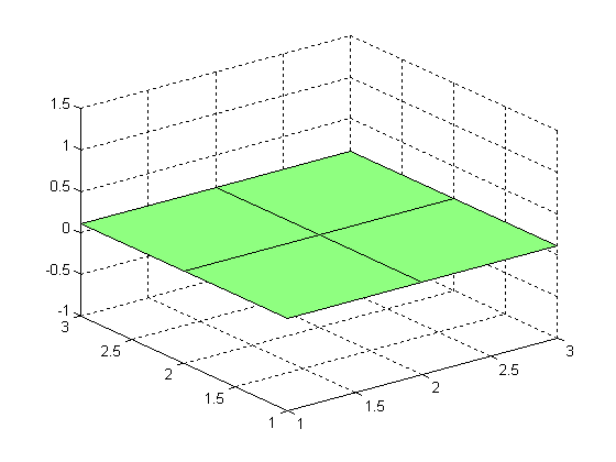
Example 2
Create
an average filter and move it over an image. Display the new
image.
Solution
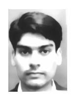
me = imread( 'zeeya2.bmp');
imagesc(me)
im = rgb2gray(me);
avfilter =
fspecial( 'average',[3
3]);
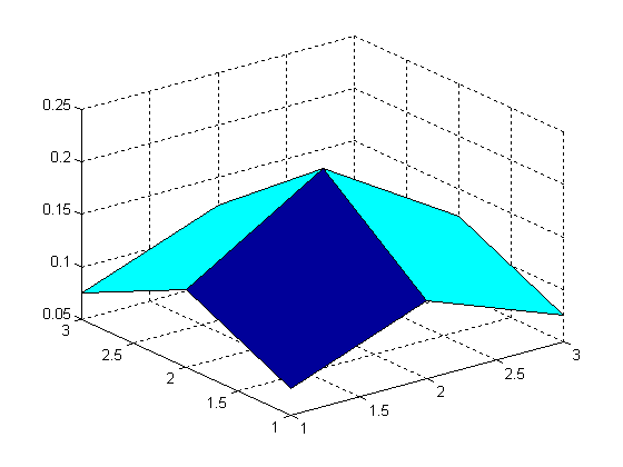
figure,
surf(avfilter);
newim=filter2(avfilter,im);
figure,
imagesc(newim);
Result
Gaussian
Smoothing
Example 3
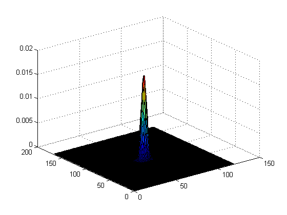
Create a Gaussian filter of 25x25 with
standard deviation 4 and repeat the above process with this
filter.
Solution
im = imread( 'testpat2.tif');
imshow(im)
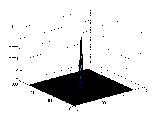
gfilter = fspecial('gaussian',[25
25],4);
figure, surf(gfilter);
newim=filter2(gfilter,im);
figure,
imagesc(newim);
Result


Gaussian
Smoothing
Example 4
Repeat above example on another image.
Solution
me = imread( 'zeeya2.bmp');
imagesc(me)
im = rgb2gray(me);
gfilter = fspecial( 'gaussian',[3
3],1);
figure,
surf(gfilter);
newim=filter2(gfilter,im);
figure,
imagesc(newim);
Result
Convolution in
Frequency Domain
Example 5
Make Gaussian filter (256x256) with standard
deviation 4. Generate 2D Fourier Transform of the filter. Read
any image and take its Fourier Transform and apply the filter
to the image by multiplying the FFT of the image and the FFT
of the filter together.
Solution
im = imread('testpat2.tif');
imshow(im)
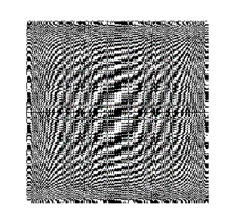
imfft=fft2(im);
%[m,n]=size(imfft)
figure,
imshow(imfft);
c=improfile(imfft);
grid
gfilter = fspecial('gaussian',[256
256],4);
figure,
surf(gfilter);
gfiltfft =
fft2(gfilter);
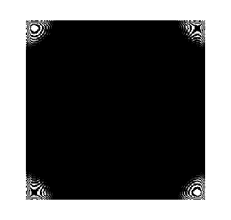
newimfft=imfft.*gfiltfft;
figure,
imshow(newimfft)
imifft=ifft2(newimfft);
figure,
imshow(imifft)
Result
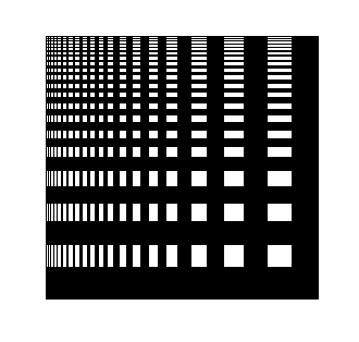
Fourier Transform of
an averaging filter
Example 7
Construct an average filter, but instead
of using the 'fspecial' function use the following commands to
construct a filter with the same size as the image(256x256 in
this case), with a (say) 21x21 square averaging region in the
middle.
Solution
avfilt = zeros(256);
avfilt(118:138, 118:138) = ones(21);
avfilt = avfilt./(sum(sum(avfilt)));
surf(avfit)
Result
Task #1
I would like the following:
a) An image of yourself, your FFT, the FFt of a
Gaussian smoothing filter, the product of your FFT and the
filter, and the final smoothed image. (Choose a Gaussian
filter standard deviation other than 4 pixels)
b) A sequence of images as above but using an
averaging filter.
c) A listing of the MATLAB commands you used to
do the above tasks (or the function/script you might have
written to do this).
Solution
me = imread( 'zeeya2.bmp');
im = rgb2gray(me);
imshow(im)
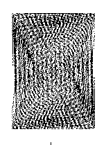
imfft=fft2(im);
figure,
imshow(imfft);
gfilter = fspecial( 'gaussian',[168
120],3);
figure,
surf(gfilter);
gfiltfft =
fft2(gfilter);
newimfft=imfft.*gfiltfft;
figure,
imshow(newimfft)
imifft=ifft2(newimfft);
figure,
imshow(imifft)
clear all
Result
Note: The IFFT of the
product of FFTs produced blank image due to only displayed
real part of complex data ( warning message displayed is
"Displaying real part of complex input")
HELP
FSPECIAL
FSPECIAL Create predefined filters.
H = FSPECIAL(TYPE) creates a two-dimensional filter H of the
specified type. (FSPECIAL returns H as a computational
molecule, which is the appropriate form to use with FILTER2.)
TYPE is a string having one of these values:
'gaussian' for a Gaussian lowpass filter
'sobel' for a Sobel horizontal edge-emphasizing filter
'prewitt' for a Prewitt horizontal edge-emphasizing
filter
'laplacian' for a filter approximating thetwo-dimensional
Laplacian operator
'log' for a Laplacian of Gaussian filter
'average' for an averaging filter
'unsharp' for an unsharp contrast enhancement filter
Depending on TYPE, FSPECIAL can take additional parameters
which you can supply. These parameters all have default
values.
H = FSPECIAL('gaussian',N,SIGMA) returns a rotationally
symmetric Gaussian lowpass filter with standard deviation
SIGMA (in pixels). N is a 1-by-2 vector specifying the number
of rows and columns in H. (N can also be a scalar, in which
case H is N-by-N.) If you do not specify the parameters,
FSPECIAL uses the default values of [3 3] for N and 0.5 for
SIGMA.
H = FSPECIAL('sobel') returns this 3-by-3 horizontal edge
finding and y-derivative approximation filter:
[1 2 1;0 0 0;-1 -2 -1].
To find vertical edges, or for x-derivates, use -h'.
H = FSPECIAL('prewitt') returns this 3-by-3 horizontal edge
finding and y-derivative approximation filter:
[1 1 1;0 0 0;-1 -1 -1].
To find vertical edges, or for x-derivates, use -h'.
H = FSPECIAL('laplacian',ALPHA) returns a 3-by-3 filter
approximating the shape of the two-dimensional Laplacian
operator. The parameter ALPHA controls the shape of the
Laplacian and must be in the range 0.0 to 1.0. FSPECIAL uses
the default value of 0.2 if you do not specify ALPHA.
H = FSPECIAL('log',N,SIGMA) returns a rotationally symmetric
Laplacian of Gaussian filter with standard deviation SIGMA (in
pixels). N is a 1-by-2 vector specifying the number of
rows and columns in H. (N can also be a scalar, in which case
H is N-by-N.) If you do not specify the parameters, FSPECIAL
uses the default values of [5 5] for N and 0.5 for SIGMA.
H = FSPECIAL('average',N) returns an averaging filter. N is a
1-by-2 vector specifying the number of rows and columns in H.
(N can also be a scalar, in which case H is N-by-N.) If you do
not specify N, FSPECIAL uses the default value of [3 3].
H = FSPECIAL('unsharp',ALPHA) returns a 3-by-3 unsharp
contrast enhancement filter. FSPECIAL creates the unsharp
filter from the negative of the Laplacian filter with
parameter ALPHA. ALPHA controls the shape of the Laplacian and
must be in the range 0.0 to 1.0. FSPECIAL uses the default
value of 0.2 if you do not specify ALPHA.
Example
I = imread('saturn.tif');
h = fspecial('unsharp',0.5);
I2 = filter2(h,I)/255;
imshow(I), figure, imshow(I2))
SURF
SURF 3-D colored surface.
SURF(X,Y,Z,C) plots the colored parametric surface defined by
four matrix arguments. The view point is specified by VIEW.
The axis labels are determined by the range of X, Y and Z, or
by the current setting of AXIS. The color scaling is
determined by the range of C, or by the current setting of
CAXIS. The scaled color values are used as indices into the
current COLORMAP. The shading model is set by SHADING.
SURF(X,Y,Z) uses C = Z, so color is proportional to surface
height.
SURF(x,y,Z) and SURF(x,y,Z,C), with two vector arguments
replacing the first two matrix arguments, must have length(x)
= n and length(y) = m where [m,n] = size(Z). In this case, the
vertices of the surface patches are the triples (x(j), y(i),
Z(i,j)). Note that x corresponds to the columns of Z and y
corresponds to the rows.
SURF(Z) and SURF(Z,C) use x = 1:n and y = 1:m. In this case,
the height, Z, is a single-valued function, defined over a
geometrically rectangular grid.
SURF(...,'PropertyName',PropertyValue,...) sets the value of
the specified surface property. Multiple property values
can be set with a single statement.
SURF returns a handle to a SURFACE object.
AXIS, CAXIS, COLORMAP, HOLD, SHADING and VIEW set figure,
axes, and surface properties which affect the display of
the surface.
FFT2
FFT2 Two-dimensional discrete Fourier
Transform.
FFT2(X) returns the two-dimensional Fourier transform of
matrix X. If X is a vector, the result will have the same
orientation.
FFT2(X,MROWS,NCOLS) pads matrix X with zeros to size
MROWS-by-NCOLS before transforming.
IFFT2
IFFT2 Two-dimensional inverse discrete
Fourier transform.
IFFT2(F) returns the two-dimensional inverse Fourier transform
of matrix F. If F is a vector, the result will have the same
orientation.
IFFT2(F,MROWS,NCOLS) pads matrix F with zeros to size
MROWS-by-NCOLS before transforming.
IMPROFILE
IMPROFILE Compute pixel-value cross-sections
along line segments.
IMPROFILE computes the intensity values along a line or a
multiline path in an image. IMPROFILE selects equally spaced
points along the path you specify, and then uses interpolation
to find the intensity value for each point. IMPROFILE works
with grayscale intensity images and RGB images.
If you call IMPROFILE with one of these syntaxes, it operates
interactively on the image in the current axes:
C = IMPROFILE
C = IMPROFILE(N)
N specifies the number of points to compute intensity values
for. If you do not provide this argument, IMPROFILE chooses a
value for N, roughly equal to the number of pixels the path
traverses.
You specify the line or path using the mouse, by clicking on
points in the image. Press <BACKSPACE> or <DELETE> to remove
the previously selected point. A shift-click, right-click, or
double-click adds a final point and ends the selection;
pressing <RETURN> finishes the selection without adding a
point. When you finish selecting points, IMPROFILE returns the
interpolated data values in C. C is an N-by-1 vector if the
input is a grayscale intensity image, or an N-by-1-by-3 array
if the input image is an RGB image.
If you omit the output argument, IMPROFILE displays a plot of
the computed intensity values. If the specified path consists
of a single line segment, IMPROFILE creates a two-dimensional
plot of intensity values versus the distance along the line
segment; if the path consists of two or more line segments,
IMPROFILE creates a three-dimensional plot of the intensity
values versus their x- and y-coordinates.
You can also specify the path noninteractively, using these
syntaxes:
C = IMPROFILE(I,xi,yi)
C = IMPROFILE(I,xi,yi,N)
xi and yi are equal-length vectors specifying the spatial
coordinates of the endpoints of the line segments.
You can use these syntaxes to return additional information:
[CX,CY,C] = IMPROFILE(...)
[CX,CY,C,xi,yi] = IMPROFILE(...)
CX and CY are vectors of length N, containing the spatial
coordinates of the points at which the intensity values are
computed.
To specify a nondefault spatial coordinate system for the
input image, use these syntaxes:
[...] = IMPROFILE(x,y,I,xi,yi)
[...] = IMPROFILE(x,y,I,xi,yi,N)
x and y are 2-element vectors specifying the image XData and
YData.
[...] = IMPROFILE(...,METHOD) uses the specified interpolation
method. METHOD is a string that can have one of these values:
'nearest' (default) uses nearest neighbor interpolation
'bilinear' uses bilinear interpolation
'bicubic' uses bicubic interpolation
If you omit the METHOD argument, IMPROFILE uses the default
method of 'nearest'.
Class Support
The input image can be of class uint8, uint16, or double.
All other inputs and outputs are of class double.
Example
I = imread('alumgrns.tif');
x = [35 338 346 103];
y = [253 250 17 148];
improfile(I,x,y), grid on
FILTER2
FILTER2 Two-dimensional digital filter.
Y = FILTER2(B,X) filters the data in X with the 2-D FIR filter
in the matrix B. The result, Y, is computed
using 2-D correlation and is the same size as X.
Y = FILTER2(B,X,'shape') returns Y computed via 2-D
correlation with size specified by 'shape':
'same' - (default) returns the central part of the
correlation that is the same size as X.
'valid' - returns only those parts of the correlation
that are computed without the zero-padded edges, size(Y) <
size(X).
'full' - returns the full 2-D correlation, size(Y) >
size(X).
FILTER2 uses CONV2 to do most of the work. 2-D correlation is
related to 2-D convolution by a 180 degree rotation of the
filter matrix.
CV
Lab 1 CV
Lab2
CV
Lab 3
CV Lab4
CV
Lab 5
CV
Lab 6
CV
Lab7 CV
Lab8
Other
material
|
|
|