The MATLAB (Matrix Lab) signal processing Toolbox has a large variety of functions for generating continuous-time and discrete time signals. In this lab, we shall learn how to generate some commonly used signals.

Generate triangular wave  using sawtooth                                                                                                                                                                                                                                     

Example 1                                                                                                                                 

 Generate a triangular wave of amplitude =1 unit, a frequency of 10л radians per second and a width of 0.5 unit.

 Solution                                                                                                                                    

    A=1

 Result                                                                                                                                       

Generate square wave                                                                                                               

Example 2                                                                                                                                 

 Generate square wave with amplitude 1, fundamental frequency 10л radian per second and duty cycle =0.5

 Solution                                                                                                                                    

     A=1

    axis([0 1 -2 2]) % this is an optional command and helps in clear visualization of the signal

Result                                                                                                                                       

Generate discrete time square wave                                                                                           

Example 3                                                                                                                                 

  Generate a discrete time square wave, with frequency л /4 radians  per second, duty cycle=0.5  and   amplitude =1 unit.

 Solution                                                                                                                                    

     A=1

    stem(n,x)

 Result                                                                                                                                       

Discrete time triangular wave                                                                                                     

Exercise 1(a)                                                                                                                             

 Generate a discrete time triangular wave of unity amplitude with width 0.5 and frequency 10л radians per second.

 Solution                                                                                                                                    

 Result                                                                                                                                        

Sinusoidal waves                                                                                                                       

Exercise 1(b)                                                                                                                             

 Draw the following sinusoidal signals:

(i) Acos(wt+Ø)     (ii) Asin(wt+Ø)

 where A=4 w=20л and Ø = 30 degrees.

 Note convert degrees into radians.

 Solution                                                                                                                                      

    %(i) Acos(wt+Ø)

 Result                                                                                                                                        

 Solution                                                                                                                                      

    %(ii) Asin(wt+Ø)

 Result                                                                                                                                        

Exponential signals                                                                                                                    

Exercise 2                                                                                                                                 

 Draw the following signals

 (a) x(t)=5e^-6t    (b) y(t)=3e^5t     (c) x[n] = 2(0.85)ⁿ       (d)  z(t) = 60sin(20л)e^-6t      (e) y[n] = 60sin(20 л n)e^-6n

 Solution                                                                                                                                      

    % 2 (a)  x(t)=5e^-6t

 Result                                                                                                                                        

 Solution                                                                                                                                      

    % 2 (b)  y(t)=3e^5t

 Result                                                                                                                                        

 Solution                                                                                                                                      

    % 2 (c)  x[n] = 2(0.85)ⁿ

 Result                                                                                                                                        

 Solution                                                                                                                                      

    % 2 (d)  z(t) = 60sin(20л)5e^-6t

 Result                                                                                                                                        

 Solution                                                                                                                                      

    % 2 (e)  y(n)=60sin(20 л n)5e^-6n 

 Result                                                                                                                                        

 Ones function                                                                                                                           

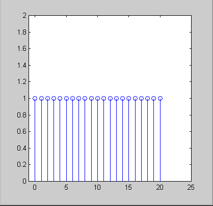
Example 4                                                                                                                                 

 A Discrete time unit step function may be created as follows

 Solution                                                                                                                                      

    n=0:1:20;

    x=ones(1,length(n));

    stem(n,x)

    axis([-1 25 0 2])  % optional

 Result                                                                                                                                        

Discrete time signals                                                                                                                  

Exercise 3a                                                                                                                               

 Draw the following discrete time functions

 a (i)  x[n] = n (ramp function)        a (ii)  x[n] = δ[n] (impulse function)

 Solution                                                                                                                                      

    % a (i)  x[n] = n (ramp function)

    n = 0:1:20;

    x = n;

    stem(n,x)

 Result                                                                                                                                        

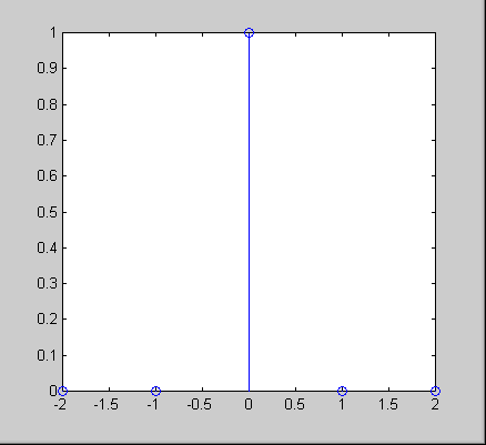
 Solution                                                                                                                                      

    % a (ii)  x[n] = δ[n] (impulse function)

    n = -2:1:2;

    x = [0 0 1 0 0];

    stem(n,x)

 Result                                                                                                                                        

Different signals                                                                                                                         

Exercise 3b                                                                                                                               

 Get help for the built -in function "sinc" and here plot sinc function (i.e. sin(x)/x) for x between -5 to 5.

 Solution                                                                                                                                      

    %  (sinc function)

    x  = -5:1:5;

    y = sinc(x);

    plot(x,y)

 Result                                                                                                                                        

Different signals                                                                                                                         

Exercise 3c                                                                                                                               

 Plot a rectangular function of width 3 units. (use built -in function "rectpuls".

 Solution                                                                                                                                      

    %  (rectpuls function)

    t  = -5:1:5;

    w =3;

    y = rectpuls(t,w)

    stem(t,y)

 Result                                                                                                                                        

Different signals                                                                                                                         

Exercise 3d                                                                                                                               

 Draw a discrete time triangular pulse using the built -in function "tripuls".

 Solution                                                                                                                                      

    %  (tripuls function)

    t  = -5:1:5;

    w =3;

    y = tripuls(t,w)

    stem(t,y)

 Result                                                                                                                                        

Different signals                                                                                                                         

Exercise 3e                                                                                                                               

 Find and plot u[n]-u[n-5], where u[n] is a discrete time unit step signal.

 Solution                                                                                                                                      

    %  (Unit step function)

    n=0:1:20;

    x=ones(1,length(n)-length(n-5));

    stem(n,x)

 Result                                                                                                                                        

Discrete time signals                                                                                                                  

Exercise 4                                                                                                                                 

 Plot the discrete time signal x[nT] = 4n/(2+n^2), T=2. On the same graph paper, plot the following:

    a.  x[nT], T=3             b.  x[nT] = 0.5

    c.  x[(n+4)T], T=2      d.  x[(n-2)T], T=0.75

 Solution                                                                                                                                      

    A=4;

 Result                                                                                                                                        

 Solution                                                                                                                                      

    % exercise 4a for T=3

    A=4;

 Result                                                                                                                                        

 Solution                                                                                                                                      

    %  exercise 4b for T=0.5

    A=4;

 Result                                                                                                                                        

 Solution                                                                                                                                      

    %  exercise 4c for x[(n+4)T,  T=2

    A=4;

 Result                                                                                                                                        

 Solution                                                                                                                                      

    %  exercise 4d for x[(n-2)T,  T=0.75

    A=4;

 Result                                                                                                                                        

Continuous time signals                                                                                                              

Exercise 5                                                                                                                                 

Plot the continuous time signals x(t) = t/t2 + 4). On the same graph pager, plot the following:

 1.  x(1.5t)      2.   x(0.8t)        3.  x(t+3.6)       4.  x(2t-1)

 Solution                                                                                                                                      

    t=-10:1:10;

 Result                                                                                                                                        

 Solution                                                                                                                                      

    %  1). x(1.5t)

    t = -10:1:10;

 Result                                                                                                                                        

 Solution                                                                                                                                      

    %  2). x(0.8t)

    t = -10:1:10;

 Result                                                                                                                                        

 Solution                                                                                                                                      

    %  3). x(t+3.6t)

    t = -10:1:10;

 Result                                                                                                                                        

 Solution                                                                                                                                      

    %  4). x(2t -1)

    t = -10:1:10;

 Result                                                                                                                                        

Continuous time signal                                                                                                               

Exercise 6                                                                                                                                 

     A=1

 HELP                                                                                                                                       

 PLOT                                                                                                                                        

 PLOT Linear plot.
PLOT(X,Y) plots vector Y versus vector X. If X or Y is a matrix, then the vector is plotted versus the rows or columns of the matrix, whichever line up. If X is a scalar and Y is a vector, length(Y) disconnected points are plotted.

 STEM                                                                                                                                      

STEM Discrete sequence or "stem" plot.
STEM(Y) plots the data sequence Y as stems from the x axis terminated with circles for the data value.
STEM(X,Y) plots the data sequence Y at the values specified in X.

 SAWTOOTH                                                                                                                              SAWTOOTH Sawtooth and triangle wave generation.
SAWTOOTH(T) generates a sawtooth wave with period 2*pi for the elements of time vector T. SAWTOOTH(T) is like SIN(T), only it creates a sawtooth wave with peaks of +1 to -1 instead of
a sine wave.
SAWTOOTH(T,WIDTH) generates a modified triangle wave where WIDTH, a scalar parameter between 0 and 1, determines the fraction between 0 and 2*pi at which the maximum occurs. The function increases from -1
to 1 on the interval 0 to WIDTH*2*pi, then decreases linearly from 1 back to -1 on the interval WIDTH*2*pi to 2*pi. Thus WIDTH = .5 gives you a triangle wave, symmetric about time instant pi with peak amplitude
of one. SAWTOOTH(T,1) is equivalent to SAWTOOTH(T).
Caution: this function is inaccurate for huge numerical inputs

 SQUARE                                                                                                                                 

  SQUARE Square wave generation.
SQUARE(T) generates a square wave with period 2*Pi for the elements of time vector T. SQUARE(T) is like SIN(T), only it creates a square wave with peaks of +1 to -1 instead of a sine wave.
SQUARE(T,DUTY) generates a square wave with specified duty cycle. The duty cycle, DUTY, is the percent of the period in which the signal is positive.
For example, generate a 30 Hz square wave:
t = 0:.0001:.0625;
y = SQUARE(2*pi*30*t);, plot(t,y)

 ONES                                                                                                                                      

ONES Ones array.
ONES(N) is an N-by-N matrix of ones.
ONES(M,N) or ONES([M,N]) is an M-by-N matrix of ones.
ONES(M,N,P,...) or ONES([M N P ...]) is an M-by-N-by-P-by-... array of ones.
ONES(SIZE(A)) is the same size as A and all ones.

 SINC                                                                                                                                       

 SINC Sin(pi*x)/(pi*x) function.
SINC(X) returns a matrix whose elements are the sinc of the elements of X, i.e.
y = sin(pi*x)/(pi*x) if x ~= 0
    = 1                         if x = = 0
where x is an element of the input matrix and y is the resultant output element.

 RECTPULS                                                                                                                             

RECTPULS Sampled aperiodic rectangle generator.
RECTPULS(T) generates samples of a continuous, aperiodic, unity-height rectangle at the points specified in array T, centered about T=0. By default, the rectangle has width 1. Note that the interval of non-zero amplitude is defined to be open on the right,
i.e., RECTPULS(-0.5)=1 while RECTPULS(0.5)=0.

RECTPULS(T,W) generates a rectangle of width W.
 TRIPULS                                                                                                                                   

 TRIPULS Sampled aperiodic triangle generator.
TRIPULS(T) generates samples of a continuous, aperiodic, unity-height triangle at the points specified in array T, centered about T=0. By default, the triangle is symmetric and has width 1.

TRIPULS(T,W) generates a triangle of width W.

TRIPULS(T,W,S) allows the triangle skew S to be adjusted. The skew parameter must be in the range -1 < S < +1, where 0 generates a symmetric triangle.

DSP Lab 1   DSP Lab2   DSP Lab 3   DSP Lab4   DSP Lab 5   DSP Lab 6   DSP Lab7  DSP Lab8  DSP Lab9  DSP Lab10   DSP Lab 11  Other material