Introduction:-

                     For designing linear phase FIR filters based on the windows Fourier Series approach, MATLAB includes the following functions for generating the windows.

W=boxcar(N)                        % Rectangular window

W=hamming(N)                     % Hamming window

W=hanning(N)                       % Von Hann window

W=kaiser(N,alpha)                % Kaiser windows

W=blackman(N)                    %Blackman window         

Hamming, Hann , Kaiser and Rectangular window                                                                      

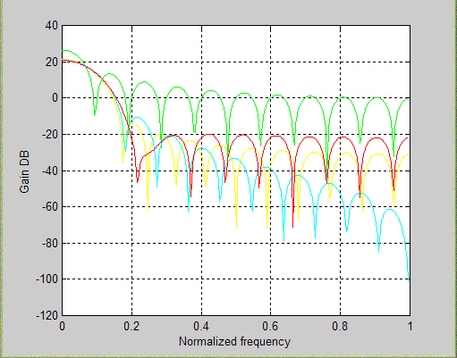
Exercise 1a                                                                                                                                

 Generate the following windows on the same graph paper. The length of each window should be 21.

Hamming, Hann, Kaiser and Rectangular windows with α = 4.5, Also sketch the magnitude responses of the above windows.

 Solution                                                                                                                                    

disp('window coefficient = ');disp(kw)

[h,omega]=freqz(kw,1,256);% frequency response of the window

mag=20*log10(abs(h)); %DB magnitude

disp('window coefficient = ');disp(kw)

[h,omega2]=freqz(kw,1,256);% frequency response of the window

mag2=20*log10(abs(h)); %DB magnitude

disp('window coefficient = ');disp(kw)

[h,omega3]=freqz(kw,1,256);% frequency response of the window

mag3=20*log10(abs(h)); %DB magnitude

disp('window coefficient = ');disp(kw)

[h,omega4]=freqz(kw,1,256);% frequency response of the window

mag4=20*log10(abs(h)); %DB magnitude

plot(omega/pi,mag,'y',omega2/pi,mag2,'g',omega3/pi,mag3,'c',omega4/pi,mag4,'r'); grid

xlabel('Normalized frequency')

ylabel('Gain DB')

Result                                                                                                                                        

window coefficient = (Kaiser Window)
0.05720440301484   0.12696179803448   0.21975935070756   0.33248311325147   0.45921890210570   0.59168070369296   0.71999582001176    0.83375532897511    0.92319479513024   0.98034599113287   1.00000000000000   0.98034599113287    0.92319479513024    0.83375532897511   0.71999582001176   0.59168070369296   0.45921890210570   0.33248311325147    0.21975935070756   0.12696179803448   0.05720440301484

window coefficient = (Rectangular window)
1  1   1   1   1   1   1   1   1   1   1   1   1   1   1   1   1   1   1   1   1

window coefficient =  (Hann window)
0.02025351319275  0.07937323358441    0.17256963302736   0.29229249349906   0.42884258086336   0.57115741913664   0.70770750650094   0.82743036697264   0.92062676641559   0.97974648680725   1.00000000000000   0.97974648680725   0.92062676641559   0.82743036697264   0.70770750650094   0.57115741913664   0.42884258086336   0.29229249349906    0.17256963302736  0.07937323358441   0.02025351319275
window coefficient = (Hamming window)
0.08000000000000  0.10251400250423  0.16785218258752  0.26961878394546  0.39785218258752  0.54000000000000   0.68214781741248  0.81038121605454  0.91214781741248  0.97748599749577  1.00000000000000  0.97748599749577  0.91214781741248  0.81038121605454  0.68214781741248  0.54000000000000  0.39785218258752  0.26961878394546  0.16785218258752  0.10251400250423  0.08000000000000

Kaiser window                                                                                                                           

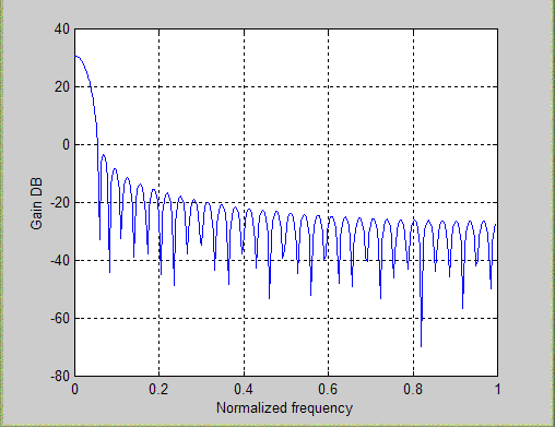
Exercise 1b                                                                                                                                

 .Generate coefficients of the Kaiser window having α = 4.5, and length 61.

Also plot the dB magnitude response of the window...

 Solution                                                                                                                                    

disp('window coefficient = ');disp(kw)

[h,omega]=freqz(kw,1,256);% frequency response of the window

mag=20*log10(abs(h)); %DB magnitude

xlabel('Normalized frequency')

ylabel('Gain DB')       

Result                                                                                                                                        

Low-pass filter using Kaiser window                                                                                           

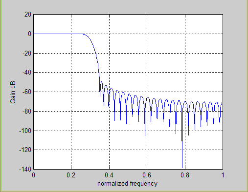
Exercise 1c                                                                                                                                

 Design a low-pass filter using the Kaiser window given above. The cutoff frequency is 0.3л

 Solution                                                                                                                                    

xlabel('normalized frequency')

ylabel('Gain dB')

Result                                                                                                                                        

window coefficient =
0.0572  0.0778  0.1011  0.1270  0.1554  0.1864  0.2198  0.2554  0.2930  0.3325  0.3735  0.4159  0.4592  0.5032  0.5475  0.5917  0.6354  0.6783  0.7200  0.7600  0.7981  0.8338  0.8667   0.8966  0.9232  0.9462   0.9653  0.9803  0.9912   0.9978  1.0000  0.9978  0.9912  0.9803   0.9653  0.9462  0.9232  0.8966  0.8667  0.8338  0.7981   0.7600  0.7200  0.6783  0.6354  0.5917  0.5475   0.5032  0.4592  0.4159  0.3735  0.3325  0.2930  0.2554  0.2198  0.1864  0.1554  0.1270   0.1011  0.0778  0.0572 

 Assignment                                                                                                                                

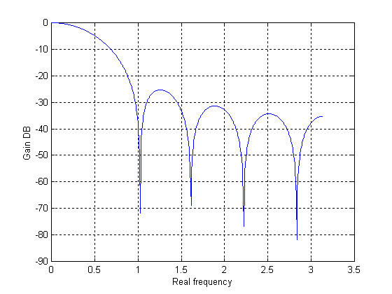
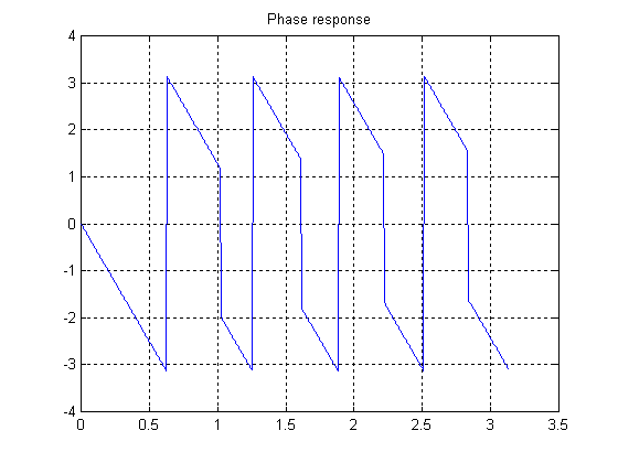
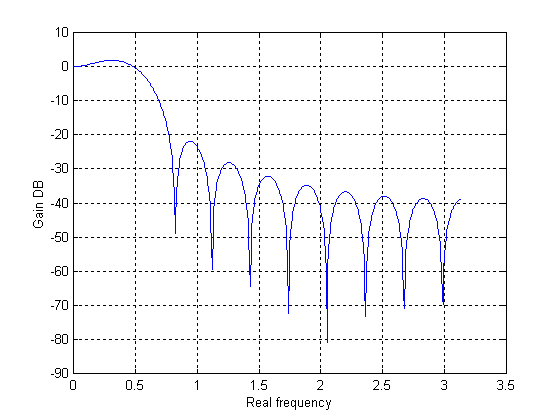
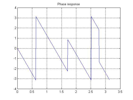
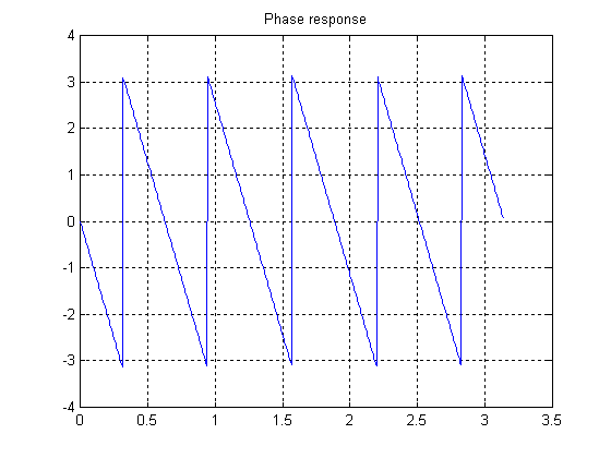
 Records of this assignment are to be submitted by October 20,2003. The record should comprise MATLAB documents, filter coefficients, plots and any separate sheets showing hand calculations etc.

 Design the following FIR filters for a sampling frequency of 50 kHz.

a) low-pass, cut-off frequency = 5 kHz, length =11, rectangular window

b) low-pass, cut-off frequency = 5 kHz, length =21, rectangular window

c) low-pass, cut-off frequency = 5 kHz, length =11, Hamming  window

d) low-pass, cut-off frequency = 2 kHz, length =21, rectangular window or Hamming window

  In each case find the filter coefficients, measure the magnitude and phase responses and comment. Plot the magnitude and phase versus real frequency f in Hz.

Solution                                                                                                                                     

Result                                                                                                                                        

Filter coefficient

b =

0.00000000000000   0.03989988227886   0.08607915423243        0.12911873134864   0.15959952911546 0.17060540604922 0.15959952911546   0.12911873134864   0.08607915423243   0.03989988227886   0.00000000000000

Window coefficient 

1     1     1     1     1     1     1     1     1     1     1

Comments:

Cut-off frequency given is 5kHz = 0.2 radians/sec (shown in freq. response figure)...................ok

Ripples are observed at less than -20dB....................................ok

In Phase response we observe linear responses......................ok

Which show that overall response is satisfactory.

Solution                                                                                                                                     

N=21;

kw=boxcar(N);

b=fir1(20,0.2,kw)

disp('window coefficient = ');disp(kw)

[h,f]=freqz(b,1,512);% frequency response of the window

mag=20*log10(abs(h));  %DB magnitude

plot(f,mag); grid

xlabel('Real frequency')

ylabel('Gain DB')

% Phase response

phase = angle(h);

figure; plot(f,phase);

title(‘Phase response’); grid

Result                                                                                                                                        

Filter coefficient

b =

-0.00000000000000  -0.02294108966990  -0.04175939567796  -0.04772502363195 -0.03441163450485   0.00000000000000   0.05161745175727   0.11135838847456     0.16703758271184   0.20646980702907   0.22070782702384   0.20646980702907  0.16703758271184      0.11135838847456   0.05161745175727   0.00000000000000 -0.03441163450485  -0.04772502363195     -0.04175939567796  -0.02294108966990

-0.00000000000000

Window coefficient 

1     1     1     1     1     1     1     1     1     1     1     1     1     1     1     1     1     1     1     1     1

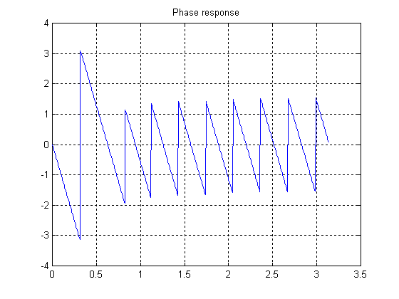
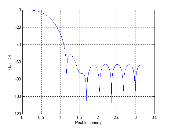
Comments:

Cut-off frequency given is 5kHz = 0.2 radians/sec (shown in freq. response figure)...................ok

Ripples are observed at less than -20dB....................................ok

In Phase response we observe linear responses......................ok

Which show that overall response is satisfactory.

Solution                                                                                                                                        % c) Low-pass, cut-off frequency=5kHz, length=11, Hamming window

N=11;

kw=hamming(N);

b=fir1(10,0.2,kw)

disp('window coefficient = ');disp(kw)

[h,f]=freqz(b,1,512);% frequency response of the window

mag=20*log10(abs(h));  %DB magnitude

plot(f,mag); grid

xlabel('Real frequency')

ylabel('Gain DB')

% Phase response

phase = angle(h);

figure; plot(f,phase);

title(‘Phase response’); grid

Result                                                                                                                                        

Filter coefficient

b =

0.00000000000000   0.00930428314502   0.04757776613442   0.12236354636114   0.20224655842984   0.23701569185916   0.20224655842984   0.12236354636114   04757776613442      0.00930428314502   0.00000000000000

Window coefficient 

0.08000000000000   0.16785218258752   0.39785218258752   0.68214781741248   0.91214781741248   1.00000000000000   0.91214781741248   0.68214781741248   0.39785218258752   0.16785218258752   0.08000000000000

Comments: 

Cut-off frequency given is 5kHz = 0.2 radians/sec (shown in freq. response figure)...................ok

Ripples are observed at less than -45dB....................................ok

In Phase response we observe linear responses......................ok

Which show that overall response is satisfactory.

Solution                                                                                                                                         % d) Low-pass, cut-off frequency=5kHz, length=21, Hamming window

N=21;

kw=hamming(N);

b=fir1(20,0.2,kw)

disp('window coefficient = ');disp(kw)

[h,f]=freqz(b,1,512);% frequency response of the window

mag=20*log10(abs(h));  %DB magnitude

plot(f,mag); grid

xlabel('Real frequency')

ylabel('Gain DB')

% Phase response

phase = angle(h);

figure; plot(f,phase);

title(‘Phase response’); grid

Result                                                                                                                                        

Filter coefficient

b =

-0.00000000000000  -0.00212227114883  -0.00632535399151  -0.01161181037762  -0.01235465674898   0.00000000000000   0.03177449755857   0.08143590756422   0.13749378170194   0.18212549038873   0.19916883010696   0.18212549038873   0.13749378170194   0.08143590756422   0.03177449755857   0.00000000000000  -0.01235465674898  -0.01161181037762  -0.00632535399151  -0.00212227114883

-0.00000000000000

Window coefficient 

0.08000000000000   0.10251400250423   0.16785218258752   0.26961878394546  0.39785218258752   0.54000000000000   0.68214781741248   0.81038121605454   0.91214781741248   0.97748599749577   1.00000000000000   0.97748599749577   0.91214781741248   0.81038121605454   0.68214781741248   0.54000000000000   0.39785218258752   0.26961878394546   0.16785218258752   0.10251400250423

0.08000000000000

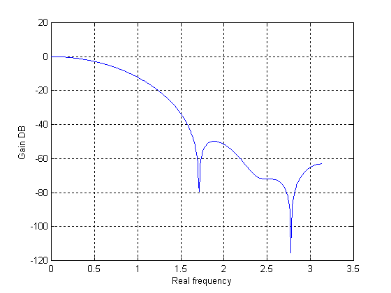
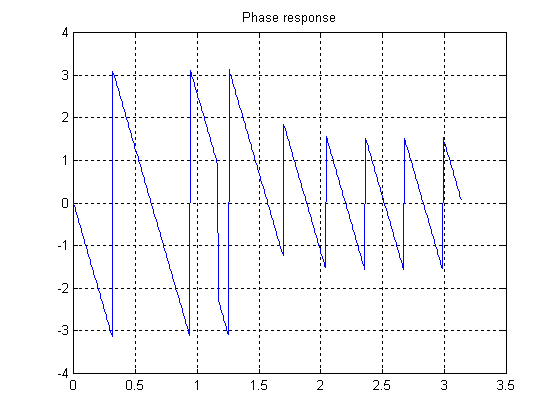
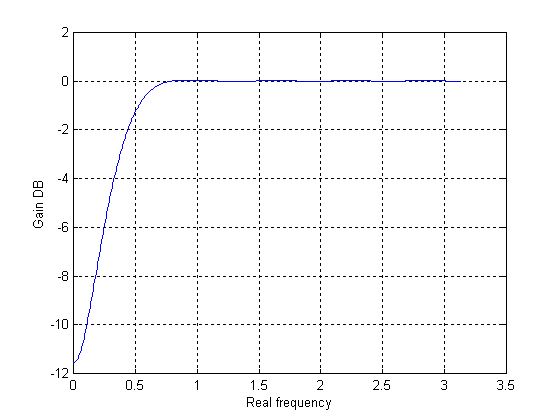
Comments:

Cut-off frequency given is 5kHz = 0.2 radians/sec (shown in freq. response figure)....................ok

Ripples are observed at less than -45dB....................................ok

In Phase response we observe linear responses......................ok

Which show that overall response is satisfactory.

Solution                                                                                                                                     

% e) High-pass, cut-off frequency=2kHz, length=21, rectangular or Hamming window

N=21;

K=hamming(N);

b=fir1(20,0.08,'high',K)

disp('window coefficient = ');disp(K)

[h,f]=freqz(b,1,512);% frequency response of the window

mag=20*log10(abs(h));  %DB magnitude

plot(f,mag); grid

xlabel('Real frequency')

ylabel('Gain DB')

% Phase response

phase = angle(h);

figure; plot(f,phase);

title(‘Phase response’); grid

Result                                                                                                                                        

Filter coefficient

b =

-0.00149859740898  -0.00279702979844  -0.00605032755780  -0.01205776784693  -0.02109060179694  -0.03273455083304  -0.04588872182864  -0.05893153521827   -0.07002233166961  -0.07747203700778   0.92111531911503  -0.07747203700778  -0.07002233166961  -0.05893153521827  -0.04588872182864  -0.03273455083304  -0.02109060179694  -0.01205776784693  -0.00605032755780  -0.00279702979844

-0.00149859740898

Window coefficient 

0.08000000000000   0.10251400250423   0.16785218258752   0.26961878394546   0.39785218258752   0.54000000000000   0.68214781741248   0.81038121605454   0.91214781741248   0.97748599749577   1.00000000000000   0.97748599749577   0.91214781741248   0.81038121605454   0.68214781741248   0.54000000000000   0.39785218258752   0.26961878394546   0.16785218258752   0.10251400250423

0.08000000000000

Comments:

Cut-off frequency given is 2kHz = 0.08 radians/sec (shown in freq. response figure).............ok

Ripples are observed are negligible ............................................ok

In Phase response we observe linear responses......................ok

Which show that overall response is satisfactory.

 HELP                                                                                                                                       

 KAISER                                                                                                                                   

 KAISER Kaiser window.
W = KAISER(N,beta) returns the BETA-valued N-point Kaiser window.

 HAMMING                                                                                                                             

HAMMING Hamming window.
HAMMING(N) returns the N-point symmetric Hamming window in a column vector.

HAMMING(N,SFLAG) generates the N-point Hamming window using SFLAG window sampling. SFLAG may be either 'symmetric' or 'periodic'. By default, a symmetric window is returned.

 HANNING                                                                                                                              

  HANNING Hanning window.
HANNING(N) returns the N-point symmetric Hanning window in a column vector. Note that the first and last zero-weighted window samples are not included.
HANNING(N,'symmetric') returns the same result as HANNING(N).
HANNING(N,'periodic') returns the N-point periodic Hanning window, and includes the first zero-weighted window sample.
NOTE: Use the HANN function to get a Hanning window which has the first and last zero-weighted samples.

 BLACKMAN                                                                                                                            

BLACKMAN Blackman window.
BLACKMAN(N) returns the N-point symmetric Blackman window in a column vector.
BLACKMAN(N,SFLAG) generates the N-point Blackman window using SFLAG window sampling. SFLAG may be either 'symmetric' or 'periodic'. By default, a symmetric window is returned.

 BOXCAR                                                                                                                                 

 BOXCAR Boxcar window.
W = BOXCAR(N) returns the N-point rectangular window.

DSP Lab 1   DSP Lab2   DSP Lab 3   DSP Lab4   DSP Lab 5   DSP Lab 6   DSP Lab7  DSP Lab8  DSP Lab9  DSP Lab10    Other material