Butterworth Filter                                                                                                                       

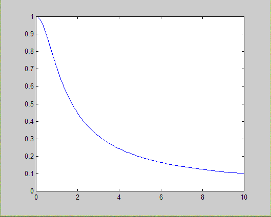
Example 1                                                                                                                                  

Find the transfer function of a first order Butterworth filter w_n = 1 radian per second.

 Solution                                                                                                                                    

   [num,den] = butter(1,1,'s');  % butter(order,cut-off frequency,'s plane')

    printsys(num,den)

    % The magnitude response of the filter can now be computed as follows:

    [y,w] = freqs(num,den);  % generates frequency response vector y and a frequency vector w

    y1 = abs(y);                       % magnitude response of the filter

    plot(w,y1)

 Result                                                                                                                                       

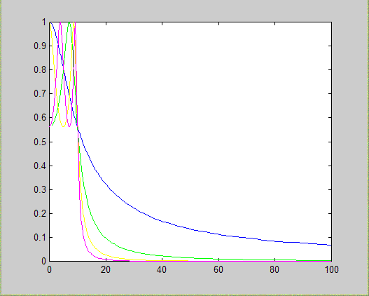
Magnitude response of different order                                                                                         

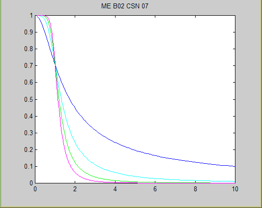
Exercise 1a                                                                                                                                

 Using the built in function "hold-on" or otherwise, compute the magnitude response of first order (as compared above), second order, third order and fourth order low pass Butterworth filter with cut-off frequency of 1 radian per second. All plots must appear on the same paper. Print your Roll No. on top of the graph paper.

 Solution                                                                                                                                    

   [num,den]=butter(1,1,'s');

    [num2,den2]=butter(2,1,'s');

    [num3,den3]=butter(3,1,'s');

    [num4,den4]=butter(4,1,'s');

    plot(w,y1,'b',w2,y2,'c',w3,y3,'g',w4,y4,'m')

Result                                                                                                                                        

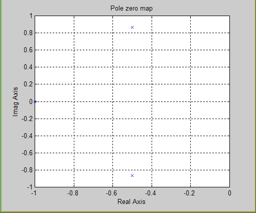
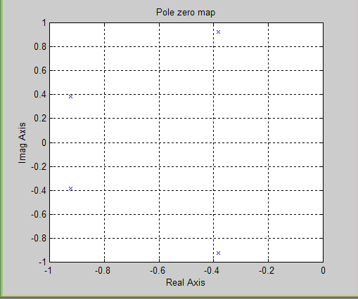
Poles and Zeros                                                                                                                         

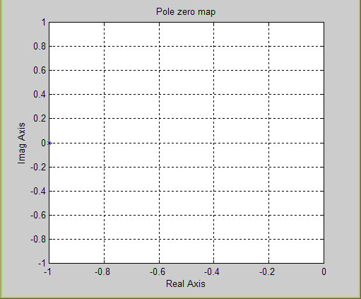
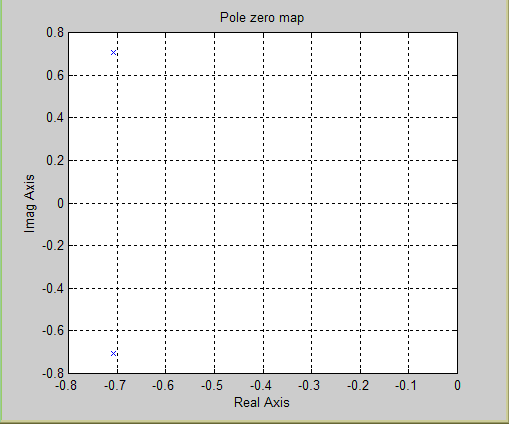
Exercise 1b                                                                                                                                

 Find Poles and Zeros of all of the above filters and plot them (separate graph for each filter) onto the s-plane.

 Solution                                                                                                                                    

    [num,den]=butter(1,1,'s');

    [num2,den2]=butter(2,1,'s');

    [num3,den3]=butter(3,1,'s');

    [num4,den4]=butter(4,1,'s');

Result                                                                                                                                        

Magnitude response of a normalized 1st, 2nd, 3rd, high pass Butterworth filter                            

Exercise 1c                                                                                                                                

 Use on-line help to plot the magnitude response of a normalized first-order, second-order, third-order high-pass Butterworth filter.

 Solution                                                                                                                                    

Result                                                                                                                                        

Band stop Butterworth filter                                                                                                        

Exercise 1d                                                                                                                                

 Repeat 1(c) for a band-stop Butterworth filter. Choose a range of frequencies (to be stopped) on your own choice.

 Solution                                                                                                                                    

Result                                                                                                                                        

Chebyshev Filter                                                                                                                        

Example 2                                                                                                                                  

 The transfer function of a low-pass type 1 Chebyshev filter of order 1 with cut off frequency 1 radian/sec and a ripple of 0.5 dB in passband can be determined as follows:

Solution                                                                                                                                     

    [num,den]=cheby1(1,0.5,1,'s');

    disp('The Transfer Function of the filter is')

Result                                                                                                                                        

Chebyshev Filter                                                                                                                        

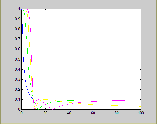
Exercise 2a                                                                                                                                

 Sketch the magnitude and phase response of a first-order, second-order, third-order and fourth-order type 1 lowpass Chebyshev filter with passband edge frequency of 10 radian/sec and passband ripple of 5 dB. Investigate the effect of changing order on the magnitude response of the system.

 Solution                                                                                                                                    

    [num,den]=cheby1(1,5,10,'s');

    disp('The Transfer Function of the filter is')

    [num,den]=cheby1(2,5,10,'s');

    disp('The Transfer Function of the filter is')

    [num,den]=cheby1(3,5,10,'s');

    disp('The Transfer Function of the filter is')

    [num,den]=cheby1(4,5,10,'s');

    disp('The Transfer Function of the filter is')

    plot(w1,y1,'b',w2,y2,'g',w3,y3,'y',w4,y4,'m')

    plot(w1,pha1,'b',w2,pha2,'g',w3,pha3,'y',w4,pha4,'m')

Result                                                                                                                                        

Chebyshev Filter                                                                                                                        

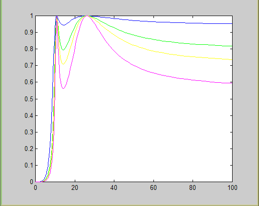
Exercise 2b                                                                                                                                 

 Draw the magnitude response of a third order lowpass type1 Chebyshev filter when the passband ripple is 0.5 db, 1 db, 2 db, 3.5 db and 5 db. What is the effect of the changing passband ripple  on the magnitude response.

 Solution                                                                                                                                    

    [num,den]=cheby1(3,0.5,10,'s'); % let passband edge frequency is 10 rad/sec

    disp('The Transfer Function of the filter is')

    %

    [num,den]=cheby1(3,1,10,'s');

    disp('The Transfer Function of the filter is')

    %

    [num,den]=cheby1(3,2,10,'s');

    disp('The Transfer Function of the filter is')

    %

    [num,den]=cheby1(3,3.5,10,'s');

    disp('The Transfer Function of the filter is')

    %

    [num,den]=cheby1(3,5,10,'s');

    disp('The Transfer Function of the filter is')

    plot(w2,y1,'b',w2,y2,'g',w3,y3,'y',w4,y4,'m',w5,y5,'c') 

Result                                                                                                                                        

 As we are increasing passband ripple, ripple is increasing in the figure.

Chebyshev Filter                                                                                                                        

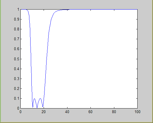
Exercise 2c                                                                                                                                

 Sketch magnitude response of a third order band-stop type1 low-pass filter which stops frequencies from 5 radian per second to 15 radian per second and allow all other frequencies to pass.

 Solution                                                                                                                                    

    [num,den]=cheby1(3,2,[5 15],'stop','s');

    disp('The Transfer Function of the filter is')

Result                                                                                                                                          

Chebyshev Filter                                                                                                                        

Exercise 2d                                                                                                                                

 Plot magnitude response of a fourth order high pass type1 Chebshev filter with passband ripple of 0.5 db, 2 db, 3db and 5db which rejects all frequencies below 10 radians per second.

 Solution                                                                                                                                    

    [num,den]=cheby1(4,0.5,10,'high','s');

    disp('The Transfer Function of the filter is')

    [num,den]=cheby1(4,2,10,'high','s');

    disp('The Transfer Function of the filter is')

    [num,den]=cheby1(4,3,10,'high','s');

    disp('The Transfer Function of the filter is')

    [num,den]=cheby1(4,5,10,'high','s');

    disp('The Transfer Function of the filter is')

    plot(w1,y1,'b',w2,y2,'g',w3,y3,'y',w4,y4,'m')

Result                                                                                                                                        

Chebyshev Filter type 2                                                                                                              

Exercise 3a                                                                                                                                

 Draw magnitude response of a first-order, second-order, third-order and fourth-order low-pass band edge frequency of 10 radians/sec and pass-band ripple of 20 dB.

 Solution                                                                                                                                    

    [num,den]=cheby2(1,20,10,'s');

    disp('The Transfer Function of the filter is')

    [num,den]=cheby2(2,20,10,'s');

    disp('The Transfer Function of the filter is')

    [num,den]=cheby2(3,20,10,'s');

    disp('The Transfer Function of the filter is')

    [num,den]=cheby2(4,20,10,'s');

    disp('The Transfer Function of the filter is')

    plot(w1,y1,'b',w2,y2,'g',w3,y3,'y',w4,y4,'m')

Result                                                                                                                                        

Chebyshev Filter type 2                                                                                                              

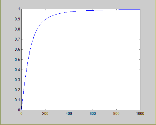
Exercise 3b                                                                                                                                

 Draw a high pass type 2 Chebyshev filter which rejects all frequencies below 10 radians per second. Take a ripple = 20 dB.

 Solution                                                                                                                                    

    [num,den]=cheby2(1,20,10,'high','s');

    disp('The Transfer Function of the filter is')

Result                                                                                                                                        

Chebyshev Filter type 2                                                                                                              

Exercise 3b                                                                                                                                

  Sketch magnitude response of a third order type 2 band stop filter with passband ripple of 20dB which stops frequencies from 10 to 20 radians per second and allows all other frequencies to pass.

 Solution                                                                                                                                    

    [num,den]=cheby2(3,20,[10 20],'stop','s');

    disp('The Transfer Function of the filter is')

Result                                                                                                                                        

 HELP                                                                                                                                       

 BUTTER                                                                                                                                  

BUTTER Butterworth digital and analog filter design.
[B,A] = BUTTER(N,Wn) designs an Nth order lowpass digital Butterworth filter and returns the filter coefficients in length N+1 vectors B (numerator) and A (denominator). The coefficients  are listed in descending powers of z. The cut-off frequency Wn must be 0.0 < Wn < 1.0, with 1.0 corresponding to half the sample rate.
If Wn is a two-element vector, Wn = [W1 W2], BUTTER returns an order 2N bandpass filter with passband W1 < W < W2.
[B,A] = BUTTER(N,Wn,'high') designs a highpass filter.
[B,A] = BUTTER(N,Wn,'stop') is a bandstop filter if Wn = [W1 W2].
When used with three left-hand arguments, as in [Z,P,K] = BUTTER(...), the zeros and poles are returned in
length N column vectors Z and P, and the gain in scalar K.
When used with four left-hand arguments, as in [A,B,C,D] = BUTTER(...), state-space matrices are returned.
BUTTER(N,Wn,'s'), BUTTER(N,Wn,'high','s') and BUTTER(N,Wn,'stop','s') design analog Butterworth filters. In this case, Wn can be bigger than 1.0.

 FREQS                                                                                                                                    

FREQS Laplace-transform (s-domain) frequency response.
H = FREQS(B,A,W) returns the complex frequency response vector H of the filter B/A:
                           nb-1      nb-2
          B(s)     b(1)s + b(2)s + ... + b(nb)
H(s) = ---- = --------------------------------
                            na-1       na-2
         A(s)      a(1)s + a(2)s + ... + a(na)

given the numerator and denominator coefficients in vectors B and A. The frequency response is evaluated at the points specified in vector W. The magnitude and phase can be graphed by calling FREQS(B,A,W) with no output arguments.
[H,W] = FREQS(B,A) automatically picks a set of 200 frequencies W on  which the frequency response is computed. FREQS(B,A,N) picks N frequencies.

 CHEBY1                                                                                                                                   

 CHEBY1 Chebyshev type I digital and analog filter design.
[B,A] = CHEBY1(N,R,Wn) designs an Nth order lowpass digital Chebyshev filter with R decibels of ripple in the passband. CHEBY1 returns the filter coefficients in length N+1 vectors  B (numerator) and A (denominator). The cut-off frequency Wn must be 0.0 < Wn < 1.0, with 1.0 corresponding to half the  sample rate. Use R=0.5 as a starting point, if you are unsure about choosing R.
If Wn is a two-element vector, Wn = [W1 W2], CHEBY1 returns an order 2N bandpass filter with passband W1 < W < W2.
[B,A] = CHEBY1(N,R,Wn,'high') designs a highpass filter.
[B,A] = CHEBY1(N,R,Wn,'stop') is a bandstop filter if Wn = [W1 W2].

When used wit h three left-hand arguments, as in [Z,P,K] = CHEBY1(...), the zeros and poles are returned in length N column vectors Z and P, and the gain in scalar K.

When used with four left-hand arguments, as in [A,B,C,D] = CHEBY1(...), state-space matrices are returned.

CHEBY1(N,R,Wn,'s'), CHEBY1(N,R,Wn,'high','s') and CHEBY1(N,R,Wn,'stop','s') design analog Chebyshev Type I filters. In this case, Wn can be bigger than 1.0.

 CHEBY2                                                                                                                                  

 CHEBY2 Chebyshev type II digital and analog filter design.
[B,A] = CHEBY2(N,R,Wn) designs an Nth order lowpass digital Chebyshev filter with the stopband ripple R decibels down and stopband edge frequency Wn. CHEBY2 returns the filter  coefficients in length N+1 vectors B (numerator) and A (denominator). The cut-off frequency Wn must be 0.0 < Wn < 1.0, with 1.0 corresponding to half the sample rate. Use R = 20 as a starting point,  if you are unsure about choosing R.

If Wn is a two-element vector, Wn = [W1 W2], CHEBY2 returns an order 2N bandpass filter with passband W1 < W < W2.
[B,A] = CHEBY2(N,R,Wn,'high') designs a highpass filter.
[B,A] = CHEBY2(N,R,Wn,'stop') is a bandstop filter if Wn = [W1 W2].

When used with three left-hand arguments, as in [Z,P,K] = CHEBY2(...), the zeros and poles are returned in
length N column vectors Z and P, and the gain in scalar K.

When used with four left-hand arguments, as in [A,B,C,D] = CHEBY2(...), state-space matrices are returned.

CHEBY2(N,R,Wn,'s'), CHEBY2(N,R,Wn,'high','s') and CHEBY2(N,R,Wn,'stop','s') design analog Chebyshev Type II filters. In this case, Wn can be bigger than 1.0.

 HOLD                                                                                                                                      

HOLD Hold current graph.
HOLD ON holds the current plot and all axis properties so that subsequent graphing commands add to the existing graph. HOLD OFF returns to the default mode whereby PLOT commands erase  the previous plots and reset all axis properties before drawing new plots.
HOLD, by itself, toggles the hold state.
HOLD does not affect axis auto ranging properties.

Algorithm note:
HOLD ON sets the Next Plot property of the current figure and axes to "add".
HOLD OFF sets the Next Plot property of the current axes to "replace".

DSP Lab 1   DSP Lab2   DSP Lab 3   DSP Lab4   DSP Lab 5   DSP Lab 6   DSP Lab7  DSP Lab8  DSP Lab9  DSP Lab10    Other material