For Schlieren technique, we can use
Eq. (3.34),
in order to evaluate the power spectrum ![]() of the signal
of the signal
![]() :
:
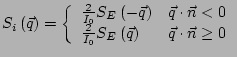 |
(3.72) |
Once the dimension of the image has been selected, in order to
observe an interesting range of wavevectors, the diameter of the
sample must fulfill the condition expressed by Eq.
(3.64), as in ONFS and ENFS,
but in this case
there's no limitation on ![]() . The diameter will be, in general,
sufficient to give a good statistical sample of the particles
we are measuring;
. The diameter will be, in general,
sufficient to give a good statistical sample of the particles
we are measuring; ![]() will be as small as we can.
will be as small as we can.
In general, for a thick sample, some of the objects will be too small, or too far from the focal plane, to be completely resolved. But their presence will prodece a speckle field, analogous to that of NFS. We will call this technique Schlieren-like Near Fiels Speckles, since it behaves like a true Schlieren technique only for big objects in the focal plane, while for the other cases it allows to measure the statistical properties of a speckle field.
Equation (3.74)
must be compared with Eq.
(3.45), that
holds for values of ![]() much less than those imposed by Eq.
(3.62), and without the blade.
The oscillations in the
sensibility of shadowgraph technique come from the non vanishing of
much less than those imposed by Eq.
(3.62), and without the blade.
The oscillations in the
sensibility of shadowgraph technique come from the non vanishing of
![]() correlations, essentially due to the phase relation
of the beams scattered at symmetric angles by a thin sample. In
SNFS, the phase relation is destroied, because one of the beams
scattered at symmetric angles is stopped.
correlations, essentially due to the phase relation
of the beams scattered at symmetric angles by a thin sample. In
SNFS, the phase relation is destroied, because one of the beams
scattered at symmetric angles is stopped.
![$\displaystyle I\left[Q\left(\vec{q}\right)\right] = \frac{1}{2} I_0 S_i\left(\vec{q}\right)$](img302.png)