Image forming techniques

Microscopy, in its basic form, consists in forming an image of a plane on a device which measures light intensity, such as a photographic film or a CCD sensor. Generally it is used to obtain informations about the intensity of the transmitted light, for example, in the case of an organic tissue, treated by some dye.

If a microscope objective forms the image of a plane on the CCD, the image is given by the interference of the transmitted and the scattered beams. For such an image, the signal can be defined as the difference of the measured intensity $I\left(\vec{x}\right)$ and the transmitted beam intensity $I_0$, divided by $I_0$. We will call this signal $i_{shadowgraph}$, for reasons that will be clear later. We consider the case in which the scattered beams are much less intense than the transmitted one. At the first order in $\delta E$, the signal is:

$$i_{shadowgraph}\left(\vec{x}\right)=\frac{I\left(\vec{x}\right)-I_0}{I_0}= \frac{2}{I_0}\Re\left[E_0 \delta E^*\left(\vec{x}\right)\right]$$ (3.21)

and the Fourier transform is:

$$i_{shadowgraph}\left(\vec{q}\right)= \frac{1}{I_0}\left[E_0 \delta E^*\left(-\vec{q}\right)+ E_0^* \delta E\left(\vec{q}\right) \right]$$ (3.22)

If the sample is transparent, and we send a plane wave through it, Eq. (3.19) tells us the value of the scattered field:

$$i_{shadowgraph}\left(\vec{q},z\right)= 2k\delta l\left(\vec{q}\right) \sin\left[\left(k-\sqrt{k^2-q^2}\right)z\right]$$ (3.23)

In order to obtain the previous result, $\delta l \left(\vec{x}\right)$ has been considered real, so that $\delta l^*\left(-\vec{q}\right) = \delta l\left(\vec{q}\right)$.

For $z=0$, that is, if the thin sample is in the focal plane, $i_{shadowgraph}\left(\vec{q},z\right)=0$. The intensity is completely uniform, and bears no informations on the sample.

Many techniques has been developed in order to make phase modulations evident: among them, holography and interferometry. A well known way to make phase modulations evident is the phase contrast microscopy. Basically, this technique consists in changing the phase of the transmitted beam by $\pi/2$. At the first order in $\delta E$:

$$i_{phase\,contrast}\left(\vec{x}\right)=\frac{I\left(\vec{x}\right)-I_0}{I_0}= \frac{2}{I_0}\Im\left[E_0^* \delta E\left(\vec{x}\right)\right]$$ (3.24)

and the Fourier transform is:

$$i_{phase\,contrast}\left(\vec{q}\right)= \frac{i}{I_0}\left[-E_0^* \delta E\left(-\vec{q}\right)+ E_0 \delta E^*\left(\vec{q}\right) \right]$$ (3.25)

Using Eq. (3.19) to evaluate the scattered field:

$$i_{phase\,contrast}\left(\vec{q},z\right)= 2k\delta l\left(\vec{q}\right) \cos\left[\left(k-\sqrt{k^2-q^2}\right)z\right]$$ (3.26)

For $z=0$, that is, with the sample in the focal plane:

$$i_{phase\,contrast}\left(\vec{q},z=0\right)= 2k\delta l\left(\vec{q}\right)$$ (3.27)

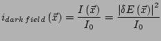
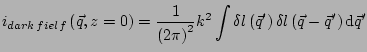
Another way to make phase modulations evident is the so called dark field technique. It consists in stopping the transmitted beam. This is accomplished by focusing the transmitted and the scattered beams by a lens, and by removing the transmitted beam by some kind of reflecting or absorbing object. This is an homodyne technique; the signal must be defined as the ratio between the measured intensity $I\left(\vec{x}\right)$ and the intensity of the transmited beam $I_0$. Since we have only $\delta E$:

$$i_{dark\,field}\left(\vec{x}\right)=\frac{I\left(\vec{x}\right)}{I_0}= \frac{\left\vert\delta E\left(\vec{x}\right)\right\vert^2}{I_0}$$ (3.28)

Equation (3.19), for $z=0$, gives:

$$i_{dark\,field}\left(\vec{x},z=0\right)=k^2 \delta l^2\left(\vec{x}\right)$$ (3.29)

In Fourier space:

$$i_{dark\,fielf}\left(\vec{q},z=0\right) = \frac{1}{\left(2\pi\rig... ...\left(\vec{q}'\right) \delta l\left(\vec{q}-\vec{q}'\right) \mathrm{d}\vec{q}'}$$ (3.30)

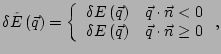
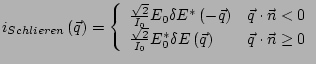
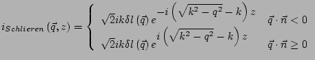
The Schlieren technique consists in focusing the beams from the sample by a lens; in the focal plane, a blade stops half of the transmitted beam, along with the beams scattered in one half plane. At the first order in $\delta E$, the signal is again, like in shadowgraph:

$$i_{Schlieren}\left(\vec{x}\right)= \frac{I\left(\vec{x}\right)-\t... ...{\tilde{I}_0}\Re\left[\tilde{E}_0 \delta \tilde{E}^*\left(\vec{x}\right)\right]$$ (3.31)

where the field $\delta \tilde{E}$ is the scattered field, without one half plane in Fourier space:

$$\delta \tilde{E}\left(\vec{q}\right)= \left\{ \begin{array}{ll} \... ...\ \delta E\left(\vec{q}\right) & \vec{q}\cdot\vec{n}\ge 0 \end{array} \right. ,$$ (3.32)

$\vec{n}$ is the vector ortogonal to the direction of the blade, $\tilde{I}_0=I_0/2$ and $\tilde{E}_0=E_0/\sqrt{2}$ are the intensity and the field of the trasmitted beam, after the blade. The Fourier transform is:

$$i_{Schlieren}\left(\vec{q}\right)= \frac{\sqrt{2}}{I_0}\left[E_0 ... ...e{E}^*\left(-\vec{q}\right)+ E_0^* \delta \tilde{E}\left(\vec{q}\right) \right]$$ (3.33)

Using Eq. (3.32):

$$i_{Schlieren}\left(\vec{q}\right)= \left\{ \begin{array}{ll} \fra... ..._0^* \delta E\left(\vec{q}\right) &\vec{q}\cdot\vec{n}\ge 0 \end{array} \right.$$ (3.34)

Using Eq. (3.19):

$$i_{Schlieren}\left(\vec{q},z\right)= \left\{ \begin{array}{ll} \s... ... i\left(\sqrt{k^2-q^2}-k\right)z} &\vec{q}\cdot\vec{n}\ge 0 \end{array} \right.$$ (3.35)

In order to obtain the previous result, $\delta l \left(\vec{x}\right)$ has been considered real, so that $\delta l^*\left(-\vec{q}\right) = \delta l\left(\vec{q}\right)$. For $z=0$, that is, if the thin sample is in the focal plane:

$$i_{Schlieren}\left(\vec{q},z=0\right)= \sqrt{2}ik \delta l\left(\vec{q}\right)$$ (3.36)

The factor $i$ means that all the Fourier components of $\delta l \left(\vec{q}\right)$ undergo a rotation of $\pi/2$: a sine-like light path modulation gives a cosine-like intensity modulation.

Hosted by www.Geocities.ws