Equations (3.23),
(3.26) and
(3.35) allow to evaluate
the evolution of the signals as ![]() , the misfocusing, is increased, for
a simple microscope objective, for phase contrast and dark field.
It should be noted that we are dealing with images formed by laser light:
as
, the misfocusing, is increased, for
a simple microscope objective, for phase contrast and dark field.
It should be noted that we are dealing with images formed by laser light:
as ![]() increases, it is possible to recover the original shape
of the observed objects; this is completely different from a white light
microscope, in which the misfocusing simply smears the images.
increases, it is possible to recover the original shape
of the observed objects; this is completely different from a white light
microscope, in which the misfocusing simply smears the images.
Equation (3.30) has not been extended
for ![]() ; in all the above mentioned techniques, however, the
variation of
; in all the above mentioned techniques, however, the
variation of ![]() strongly influences the relation between the light path
strongly influences the relation between the light path
![]() and the signal
and the signal
![]() .
This is generally a defect: thick objects, or even thin objects
dispersed in a thick volume, are difficult to be analysed. In general,
all the above mentioned techniques are applied to samples that are thin,
and in the focal plane. No improvement is obtained by misfocusing.
.
This is generally a defect: thick objects, or even thin objects
dispersed in a thick volume, are difficult to be analysed. In general,
all the above mentioned techniques are applied to samples that are thin,
and in the focal plane. No improvement is obtained by misfocusing.
A well known exception is shadograph. Shadowgraph technique consists in
sending a plane wave onto a sample,
and observing the intensity modulations generated by the sample on a
plane placed at a distance ![]() from the sample.
Using Eq. (3.23), we can derive
the transfer function
from the sample.
Using Eq. (3.23), we can derive
the transfer function
![]() of the shadowgraph technique [15,16,17]:
of the shadowgraph technique [15,16,17]:
| (3.38) |
For ![]() , the transfer function vanishes; misfocusing is needed, and is
a simple way to make phase modulations evident.
, the transfer function vanishes; misfocusing is needed, and is
a simple way to make phase modulations evident.
Looking at Eq. (3.26)
we can notice that phase contrast transfer function, as a function of ![]() ,
has a cosinusoidal behaviour:
,
has a cosinusoidal behaviour:
![$\displaystyle T_{phase\,contrast}\left(\vec{q},z\right) = 2k\cos\left[\left(k-\sqrt{k^2-q^2}\right)z\right] \approx 2k\cos\left(\frac{q^2z}{2k}\right)$](img161.png) |
(3.39) |
The shadowgraph image is created by the interference between every
scattered beam
and the transmitted beam; it's always possible, in principle, to find
the value of ![]() , in every point, simply by a
deconvolution. Shadowgraph allows the measurement of one component of
the field, which, in turns, is the convolution of the light path with
a particular function. The absolute intensity modulation of the
shadowgraph image is proportional to the mean intensity and to the
light path modulation; the constant of proportionality is the
the transfer function. The transfer function vanishes for
some wave vectors, but has maxima for other ones. At the maxima, the
sensibility equals the sensibility of phase contrast and Schlieren
techniques.
, in every point, simply by a
deconvolution. Shadowgraph allows the measurement of one component of
the field, which, in turns, is the convolution of the light path with
a particular function. The absolute intensity modulation of the
shadowgraph image is proportional to the mean intensity and to the
light path modulation; the constant of proportionality is the
the transfer function. The transfer function vanishes for
some wave vectors, but has maxima for other ones. At the maxima, the
sensibility equals the sensibility of phase contrast and Schlieren
techniques.
Now we evaluate the effect of misfocusing on a dark field microscope. We
obtain an image of a plane a distance ![]() from the cell.
Using Eq. (3.19), we can derive
the relation between the light path and the measured intensity, at a given
from the cell.
Using Eq. (3.19), we can derive
the relation between the light path and the measured intensity, at a given ![]() :
:
![$\displaystyle i_{dark\,field}\left(\vec{q},z\right) = \frac{1}{\left(2\pi\right...
...left[\sqrt{k^2-\left(\vec{q}-\vec{q}'\right)^2}-k\right]z} \mathrm{d}\vec{q}' }$](img162.png) |
(3.40) |
This expression reduces to Eq. (3.30) for
![]() . At this point, there's no appearent reason to use a misfocused
dark field instead of a focused one.
. At this point, there's no appearent reason to use a misfocused
dark field instead of a focused one.
The knowledge of
![]() , for every
, for every ![]() , can
give some informations about the spreading of the scattered light. For
the scattering of a single particle, one can measure the intensity on
planes with increasing values of
, can
give some informations about the spreading of the scattered light. For
the scattering of a single particle, one can measure the intensity on
planes with increasing values of ![]() , and calculate how fast the light
is diverging. This provides informations both on the position of the
particle and on the scattered intensity. For a sample composed by a
great number of particles, this cannot be done, and a different,
statistical approach must be applied.
, and calculate how fast the light
is diverging. This provides informations both on the position of the
particle and on the scattered intensity. For a sample composed by a
great number of particles, this cannot be done, and a different,
statistical approach must be applied.
For Schlieren technique, from Eq. (3.35):
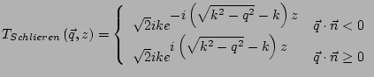 |
(3.41) |
| (3.42) |
![$\displaystyle T_{shadowgraph}\left(\vec{q},z\right) = 2k\sin\left[\left(k-\sqrt{k^2-q^2}\right)z\right] \approx 2k\sin\left(\frac{q^2z}{2k}\right)$](img159.png)