Scattered intensity and field power spectrum.

From Maxwell equations, we can derive the wave equation for a transverse component of the electric field in the vacuum [14]:

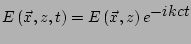
$$\frac{\partial^2}{\partial t^2} E\left(\vec{x},z,t\right) = c^2 \... ...\left(\vec{x},z,t\right) + \nabla_{\vec{x}}^2 E\left(\vec{x},z,t\right) \right]$$ (3.1)

where $\nabla_{\vec{x}}^2$ is the Laplacian oeprator, with respect to the horizontal coordinate $\vec{x}$. Since we are working with a laser, and we consider only elastic scattering, the only temporal frequency involved is $kc$:

$$E\left(\vec{x},z,t\right) = E\left(\vec{x},z\right) e^ {\displaystyle -i kct}$$ (3.2)

where $k$ is the wave vector. Eq. (3.1) becomes:

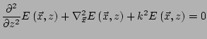$$\frac{\partial^2}{\partial z^2} E\left(\vec{x},z\right) + \nabla_{\vec{x}}^2 E\left(\vec{x},z\right) + k^2 E\left(\vec{x},z\right) = 0$$ (3.3)

We define $E_z\left(\vec{q}\right)$ as the Fourier transform of $E\left(\vec{x},z\right)$ with respect to $\vec{x}$:

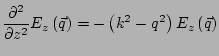$$\frac{\partial^2}{\partial z^2} E_z\left(\vec{q}\right) = -\left(k^2-q^2\right) E_z\left(\vec{q}\right)$$ (3.4)

The solution is:

$$E_z\left(\vec{q}\right) = E_0\left(\vec{q}\right) e^ {\displaystyle i \sqrt{k^2-q^2} z }$$ (3.5)

In order that this solution exists, a condition must be fulfilled:

$$q^2 < k^2,$$ (3.6)

This condition is alwais met if we consider only propagating waves.

The quantity $E_z\left(\vec{q}\right)$ is closely related to the intensity of the light crossing the plane $z=\mathrm{cost}$. Each two-dimensional Fourier mode of amplitude $E_z\left(\vec{q}\right)$, on a given $z$, and wavevector $\vec{q}$ is generated by a three-dimensional plane wave of wavevector $\left[q_x,q_y,k_z\right]$, where the only value of $k_z$ is obtained by imposing that the wavevector of any plane wave has length $k$:

$$k_z\left(q\right) = \sqrt{k^2 - q^2}$$ (3.7)

Given the values of the two-dimensional Fourier modes $E_z\left(\vec{q}\right)$ on a given $z=0$, we can evaluate $E\left(\vec{x},z\right)$ for each $\vec{x}$ and $z$, by using Eq. (3.5) and (3.7). Expressing it by its three-dimensional Fourier transform:

$$E\left(\vec{q},k_z\right)=2\pi E_0\left(\vec{q}\right) \delta \left[ k_z - k_z\left(q\right) \right]$$ (3.8)

Each three-dimensional component with amplitude $E\left(\vec{q},k_z\right)$ of the electric field represents a plane wave travelling in a different direction. We define $S_E\left(\vec{q},q_z\right)$, the two-dimensional power spectrum of $E\left(\vec{x},z\right)$:

$$\left< E_z\left(\vec{q}\right) E_z^*\left(\vec{q}'\right) \right> = \delta \left(\vec{q}-\vec{q}'\right) S_E\left(\vec{q}\right)$$ (3.9)

Light intensity, for each scattering direction, can be defined on the basis of $E\left(\vec{q},k_z\right)$:

$$\left< E\left(\vec{q},k_z\right) E^*\left(\vec{q}',k_z'\right) \r... ..._z'\right) \delta \left[k_z-k_z\left(q\right) \right] I\left(\vec{q},q_z\right)$$ (3.10)

where $I\left(\vec{q},q_z\right)$ has been expressed in terms of the transferred wavevector $\left[q_x,q_y,q_z\right]= \left[k_x,k_y,k_z\right] - \left[0,0,k\right]$. From Eq. (3.7):

$$q_z\left(\vec{q}\right) = \sqrt{k^2 - q^2} - k$$ (3.11)

Substituting $E\left(\vec{q},k_z\right)$ of Eq. (3.8) in Eq. (3.10), and comparing the result with Eq. (3.9), we can relate the scattered intensity $I\left(\vec{q},q_z\right)$ to the power spectrum of the field $S_E\left(\vec{q}\right)$:

$$I\left(\vec{q},q_z\right)=S_E\left(\vec{q}\right)$$ (3.12)

From Eq. (3.12) we notice that $I\left(q\right)$ can be measured by evaluating $E_z\left(\vec{q}\right)$ on any $z$.

If the sample is isotropic, $I\left(\vec{q},q_z\right)$ depends only on $Q=\left\vert q_x,q_y,q_z\right\vert$:

$$Q\left(q\right) = \sqrt{2}k\sqrt{1-\sqrt{1-\left(\frac{q}{k}\right)^2}}$$ (3.13)

In this case, Eq. (3.12) can be written in terms on $q$ and $Q$:

$$I\left[Q\left(q\right)\right]=S_E\left(q\right)$$ (3.14)

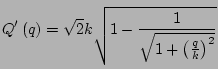
The geometrical meaning of Eq. (3.13) is explained in Fig. 3.1. For $q\ll k$, Eq. (3.13) can be approximated by $Q\left(q\right)=q$. Moreover, if Rayleigh Gans approximation holds, $I\left(q\right)$ represents the power spectrum of the refraction index of the sample. From these two considerations, we obtain the result that, for scattering on small angles and under Rayleigh Gans condition, the two dimensional correlation function of the electric field is proportional to the correlation function of the light path through the sample.

Figure 3.1: Relation between $q$ and $Q$. Geometrical interpretation of Eq. (3.13)

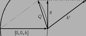Figure 3.2: Relation between the coordinate $q$ on a screen, in a far field experiment, and the transferred wave vector $Q'$. Geometrical interpretation of Eq. (3.15)

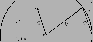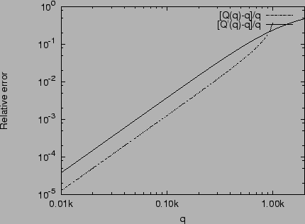
Figure 3.3: Relative error obtained neglecting the non linearity of the ralation between the sample wave vector and the near field wave vector. The graph is obtained from Eqs. (3.13) and (3.15).

When performing a far field, small angle scattering measurement, the scattered beams are focused on a screen. In suitable units, each point of the screen has a coordinate $q$. For small values of the wave vector, $q$ approximates $Q'$, the transferred wavevector. The exact relation is:

$$Q'\left(q\right) =\sqrt{2}k\sqrt{1-\frac{1}{\sqrt{1+\left(\frac{q}{k}\right)^2}}}$$ (3.15)

Equation (3.13) can be used to correct the results of a Near Field Speckles measurement. Figures 3.1 and 3.2 show the geometrical meaning of equations (3.13) and (3.15). For small values of $q$, that is $q/k\ll 1$, the two equations can be approximated with $Q=Q'=q$; the error due to this approximation is shown in Fig. 3.3: it's quite small, and it can often be neglected.

Hosted by www.Geocities.ws