5. Some problems solved by using methods of neorelativistic mechanics

Four components of the vector , having the form (4.1), give general solutions only for four functions t(t ), x₀(t ), y₀(t ), z₀(t ) from the problem of two bodies (3.8). Practically these four functions can be determined only after the function , depending on the invariant argument , where  and  as in (3.5), is found. Three functions x_AB(t ), y_AB(t ), z_AB(t ), which determine d_AB, one can obtain from (3.8) after considering three variations dx_AB(t ), dy_AB(t ), dz_AB(t ) in the functional (3.8). The corresponding vectorial differential equation for the unknown invariant vector  looks in the particular case of  as follows:

(5.1)

Here

, (5.2)

is a constant invariant vector. This  do not change in any inertial (neorelativistic) frame of reference. The equality (5.2) expresses one more neorelativistic law of conservation, that generalizes the classical second Kepler’s law. But in this new law the rate of change of the area , where , is not constant:  is changing in proportion to . If , then , but vector  in (5.2) remains constant and .

It is very important to emphasize: the second term in right part of (5.1) is Lorentz’s force (and not only in Coulomb’s field but in gravitation field also, because both are analogous from mathematical point of view). Such is the result of our “fantasy” in formulae (3.7)…

Reader can notice that in case of  (see 4.7), because of  it may occure that we will have such particle, which has zero invariant defective mass  but its intrinsic moment (spin)  will be not zero, because of  (particles like neutrino and photon).

Equations (5.1) and (5.2) show that any transformation of the seven generalised coordinates , when transformation is belonging to the abovementioned g -group, does not change anything both in vectorial or scalar magnitudes entering these equations, i.e. those magnitudes remain unchanged in any neorelativistic inertial frame of reference.

So we have got the neorelativistic form of the relativity principle (which is not declared but which naturally follows from the equations): as equations (5.1), (5.2) and (4.1) do not change both their outer appearance or their algorithmic revealing in any neorelativistic frame of reference, all real physical and mechanical processes involved in these equations do not undergo any changes as well.

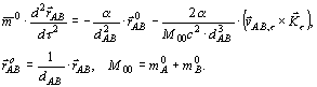
From the equality (5.1) it follows that if  by  and  being constant vectors, i.e. if  is a linear function of t , then the right part of this equality becomes equal to zero. Denoting this right invariant part  one may consider it as the interaction force between objects A and B, thus obtaining the neorelativistic generalisation of the first Newton’s law. Let us emphasize that in case of gyration vector  in (5.1) is antiparallel to . If , then  (see (5.2)) may be not so small, and in right part of (5.1) we will have . So, when radius , then interaction force is absent and velocity .

Nevertheless, together with the invariant interaction force , (right part of (5.1)) we also have to deal with two noninvariant forces of acting, namely, with the noninvariant force  representing action of object B upon object A, and with the noninvariant force  representing action of object A upon object B. In neorelativistic mechanics the three forces  and  are, generally speaking, not equal.

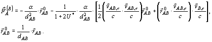
If three-dimensional noninvariant "vectors"  which one can consider in the given fixed frame of reference  (in space ), fix correspondingly material particles  and  and their center of mass  (relatively to another unit vectors  in the same space), then (as in space  also) we will have:

. (5.3)

Reckoning , taking the second derivatives of expressions (5.3), and defining  from (4.4) by , one obtains the forces  and . It appears here that

. (5.4)

Consequently, the force of action, say, , and the force of counteraction  satisfy the third Newton's law only in two cases:

1) when , i.e. when ;

2) when , i.e. in case of gyration in the problem of two bodies or two charges.

Using noninvariant "vector" of the action force , we can exact the classical expression for the Coulomb force, determining the action of an electric charge q_B upon another charge q_A, when those charges are concentrated on masses  and . If  and  then in the case of , , and according to equality , from (5.1) and (5.4) we obtain the expression:

(5.5)

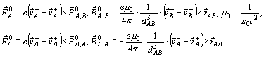
The second term in (5.5) is a correction to the usual Coulomb formula. This additional term is very small by its magnitude when  and  are small. (It is supposed here that all vectors in (5.5) are “mapped” on “our” space ). But in case of very small values of d_AB it may happen that  and . A big magnitude of the second term in (5.5) will occur when , , and . Then this additional force will be opposite to the classical Coulomb force. In such case two like charges will attract one to other. All this has also direct pertain to the problem of head-on collision of an electron beam with an analogous positron beam and also to the problem of experimental determination of the size of a particle (for instance, like in Rutherford’s experiment).

Now let us consider two unlike charges +e, -e located almost at the same point A with the difference of their velocities at the given instant  denoted as . We, for instance, may imagine a kind of a tiny "boat" A carrying a positive charge +e and a negative charge -e moving along "rails", affixed to this boat, with the corresponding velocities  and . Let analogous "boat", carrying unlike charges +e, -e, be located at the point B, and let the difference of charge velocities in B be . This gives us an image of two "elementary electric currents"  and  which are quite invariant because canon velocity  and velocity  are invariant in corresponding pseudoeucledaen spaces  (). In this "problem of four charges" the classical Coulomb force disappears completely, due to the fact that the distance between "boats" d_AB is much greater than the sizes of "boats" themselves. The corrected Coulomb formula (5.5) now explains appearing of pure magnetic interactions.

From above mentioned problem of “four charges” one can obtain two magnetic forces  and , acting between these two “boats”. These invariant vectors  and  in general case are not equal and not parallel. These magnetic forces are as follows:

(5.6) - (5.7)

They are quite analoguos to those obtained from the well-known Ampere’s formula, which describes two magnetic forces  and  acting upon two electric conductors characterized by two elemental length-vectors , and conducting electric strength currents I_A and I_B, d_AB being the distance between ,.(In Ampere’s formula element  from the first conductor has N_A ”tiny boats” and I_A = N_A i_A ; element  has N_B ”boats” with “elementary carrent” i_B, I_B = N_Bi_B). And here we mean that every positive charge  in metal conductor is concentrated on three quarks in proton, and the system of three quarks (in keeping with “confinement idea”) has common mass . Every such charge  is “statistically free”. In this case .

Here we have full coincidence between the theoretical neorelativistic solution (5.6) and experimental data thus verifying this theory. In this connection it should be reminded that the most general case of Ampere's formula cannot be confirmed by methods of classical special theory of relativity, because relativistic mechanics (STR) tries to explain phenomena of magnetism operating in its attempts to correct the classical Coulomb formula only by some scalar factors. But it can not change the direction  of usual Coulomb force in (5.5).

By using the neorelativistic law of energy conservation (4.5), was examined the model of the simplest timepiece (a linear harmonic oscillator in the form of two equal masses , joined together with an ideal spring and placed into constant gravitational field with potential function , where g₀ and R₀ are unchanged). Instead of d_AB here we can consider the invariant magnitude  . In this case the magnitude , where l₀ is a free length of the spring, determines the strain energy and the potential function , where k_c is a spring rigidity.

Neorelativistic solution of this problem is based on equality (4.5) and it reveals an usual relationship between invariant magnitudes of x(t ) and t in threedimensional pseudoeucledean space R₃ , k = 2 (because now y₀(t ) = z₀(t ) = 0 and y_AB(t ) = z_AB(t ) = 0), i.e.

. (5.8)

As one can notice, the process of changing x(t ) does not depend on the constant gravitation field with  and on the usual pseudovelocity .

But the invariant time t is, in fact, an "extrasensoric" one, and it should be noted here that in the course of the experiment one can measure only noninvariant magnitude t(t ), which in these circumstances becomes the "pseudotime", since the magnitude dt represents only the first coordinate of the invariant vector , with the magnitude  no more being constant. From the conservation law E_t = const, as in (4.2), one can derive a copmplicated enough relationship

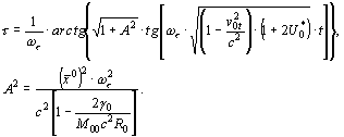(5.9)

From (5.8) and (5.9) one can eliminate invariant time  and obtain the relationship of , where

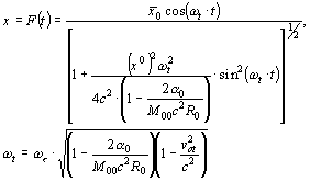(5.10)

This last function in contrast to (5.8) has a pseudoperiod , which is noninvariant and which depends on v_ot and on the gravitational field U₀,

The function x = F(t) when  (i.e. very strong gravitation) describes a process which looks like so called “pulsar”. This apparent, but nevertheless distored, pulsatory process is in agreement with modern astronomy observations. Also the pseudoperiod T_t is in full agreement both with the Pound-Rebka experiment, based upon the Moessbauer effect, and with the well-known theoretical solution offered by the Einstein general theory of relativity. (Here one only needs to find from second formula (5.10) two pseudoperiods  and , where h is the distance between two such timepices).

Thus, real invariant vibrating process (but extrasensorical one!) of the “flying” linear oscillator in constant gravitation field is determind by formula (5.8). But the inhabitans of the planet Earth with their destored sensations can “see” only noninvariant relationship in the form (5.10). Approximatly such mistake these “inhabitans” will make when during two years they wil fix the position of planet Mars among “resting” stars on a starglobe: instead of “extrasensorical” elliptic trajectory of Mars they will have quite a destored trace.

From first two equalities (4.2) one can find that . This value determines the constant (fixed) direction vector , in subspace  belonging to the space , in which we had “immersed” our mechanical problem. But the canonic velocity  of the same centre of mass M₀₀ = 2m⁰ is not uniformly because

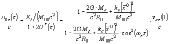, (5.11)

where

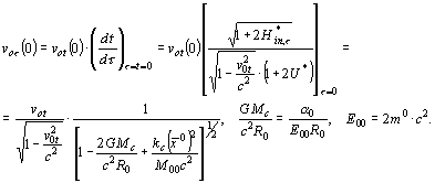(5.12)

Here M_C is the mass of body creating the constant gravitation, R₀ - is an invariant “algebraic distance” between M_C and our timepiece centre of mass, i.e. R₀ do not depend on a very small value x(t ); G - is gravitation constant. Expression (5.11) gives full information about de’Broglie vawe, which associate the little flying particle, like our flying timepiece.

We shall finish on that that the inventor of a microscope Leeuwenhoek was not a microbiologiest at all, but he was sure that his microscope showed what it showed. We expect same attitude to “the mathematical microscope” offered here.

Here are some of “pictures”, which demonstrate our “microscope” (we also include here references with Ukrainian text using label “U.t.”):

1) Neorelativistic functional of action – (3.7), (3.8) and (7.10) “U.t.”.

2) Invariant vector of energy  (in two-body problem) and its four component (they are the same for any multy-body problem) – (4.1), (4.2) and (7.19), (7.21) “U.t.”

3) Invariant Hamiltonian function – (4.5) and (7.27) “U.t.”

4) Modulus of energy vector  - (4.8) and three type of mass  – (4.7).

5) Generalized and quite invariant Newton’s equation of motion in two-body (or two charges) problem; if , then (in case of gyration) the invariant force of interaction  tends to zero; - (5.1).

6) Generalized second Kepler’s law (5.2) and linear equation of interaction (5.1).

7) Generalized magnetic and gravitional (Lorentz’s) force (the second term in right part of equality (5.1)).

8) Generalized (noninvariant) Coulomb formula – (5.5) (also in gravitational case for two masses ).

9) Ampere’s law for interaction between two “elementary currents” – (5.6), (5.7); both magnetic forces  and  are quite invariant vectors in subspace , belonging to pseudoeuclidean space , and (contrary to STR) they do not turn into electrostatic in any “mooving classical frame of reference”.

10) Interaction force  between “elementary current” and free mooving electron with velocity  - (8.5) “U.t.” (the last two terms in (8.5) do not depend on velocity ).

11) Interaction force  between two currents (loop contour), when both planes of contours are parallel to plane  and distance between their centres , and also the torque  - (8.30), (8.31) “U.t.”.

12) An ideal oscillator mooving with velocity  in gravitation fied;

ŕ) neorelativistic vibration process relatively to invariant time – (5.8);

b) relatively to nonivariant “pseudotime” t – (5.10), when “pseudoperiod” T_t depends on gravitation and velocity .

13) Oscillators “pseudoperiod” T_t and relationship  in very strong gravitation field, when , is like at so-called “pulsar” - (5.10).

14) More correct definition of Einstein’s principle of equivalence – (9.13) “U.t.”.

15) Neorelativistic verifeing of the well-known Pound-Rebka’s experiment – (9.12) “U.t.”.

16) The vibration velocity  - (5.11) of the ideal “flying oscillator”, describing de’Broglie’s vawe, which associate the mooving centre of mass.

So author (using his own intuition) had realized his main perpose: from all complications of STR and GTR – again back to usual outward appearance of classical equations and their solutions (only by changing absolute time t on invariant time t, when principle of relativity is only a logical consequence of these utterly invariant solutions). Thank goodness and God…