SNFS setup for non equilibrium fluctuation measurements.

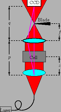
The overall system is sketched in Fig. 4.12.

Figure 4.12: The optical setupt for the measurement of non equilibrium fluctuations with SNFS.

The range $\left[q_{min},q_{max}\right]$ of the fluctuations we measure is about $\left[2\times10^3\mathrm{m}^{-1},2\times10^5\mathrm{m}^{-1}\right]$, that is, the fluctuations range from ten microns to some millimeters. By using Eqs. (4.2) and (4.5), we obtain $D\gtrapprox 10\mathrm{mm}$ and $z<125\mathrm{mm}$. The cell we used, described in Chapter 9, has an internal diameter of about $25\mathrm{mm}$.

Following Eq. (4.3), we obtain the magnification: $M=1$. We used an achromatic doublet with a $25\mathrm{mm}$ diameter and focal length $f=100\mathrm{mm}$. To obtain the required magnification, $p=q=200\mathrm{mm}$. Since SNFS is affected by small inhomogeneous fluctuations of air temperature, we choose to put the collimating lens and the objective lens as close as possible to the cell, in order to prevent air movements. This resulted in a negative $z$.

The whole optical system is shown in Fig. 4.3.

Hosted by www.Geocities.ws