Vanishing of the $\left <EE\right >$ correlations.

In Eq. (3.51) we neglected the terms like $\int \tilde{E}\left(\vec{x}\right) \tilde{E}\left(\vec{x}+\Delta \vec{x}\right) d\vec{x}$. Such terms should give contributions like $\left<E\left(\vec{x}\right) E\left(\vec{x}+\Delta \vec{x}\right)\right>$ in the Vick formulas; we neglected them assuming that the phases are random. In this section we will analyze the conditions under which this happens.

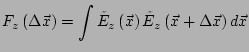
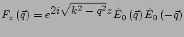
In general, $\left <EE\right >$ correlations are not negligible. For example, we can consider an opaque screen, with a transmission coefficient dependent on the position, with gaussian distribution. We know that Vick formulas hold. Now, we send a beam through it, and measure the outgoing intensity correlation function, immediately after the screen. Since all the points are in phase, we can assume that the field is real. The Vick formula for the intensity correlation function states that $C_I\left(\Delta \vec{x}\right)=\left<I\right>^2+2\left\vert C_E\left(\Delta \vec{x}\right)\right\vert^2$, due to the not negligible contribution of the term $\left <EE\right >$, which becomes equal to $\left<EE^*\right>$. Another example can be found in the theory of shadowgraph: the term $\left <EE\right >$ is responsible for the oscillations of the transfer function defined in Eq. (3.37).

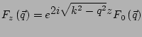
Now we derive the equations giving the evolution of $\left <EE\right >$ as $z$ increases. We define:

$$F_z\left(\Delta \vec{x}\right)= \int \tilde{E}_z\left(\vec{x}\right) \tilde{E}_z\left(\vec{x}+\Delta \vec{x}\right) d\vec{x}$$ (3.55)

The Fourier transform of $F\left(\Delta \vec{x}\right)$ is:

$$F_z\left(\vec{q}\right)= \tilde{E}_z\left(\vec{q}\right) \tilde{E}_z\left(-\vec{q}\right)$$ (3.56)

We can notice that $F\left(\vec{q}\right)$ is the power spectrum if $\tilde{E}\left(-\vec{q}\right)$ is the complex conjugate of $\tilde{E}\left(\vec{q}\right)$, that is if $\tilde{E}\left(\vec{x}\right)$ is real. By using Eq. (3.5), we obtain the evolution of $F_z\left(\vec{q}\right)$:

$$F_z\left(\vec{q}\right)=e^{\displaystyle 2i \sqrt{k^2-q^2} z } \tilde{E}_0\left(\vec{q}\right)\tilde{E}_0\left(-\vec{q}\right)$$ (3.57)

This gives the evolution equation of $F_z\left(\vec{q}\right)$:

$$F_z\left(\vec{q}\right)=e^{\displaystyle 2i \sqrt{k^2-q^2} z } F_0\left(\vec{q}\right)$$ (3.58)

Comparing this equation with Eq. (3.5), we see that $F_z\left(\vec{q}\right)$ evolves like the electric field $E_z\left(\vec{q}\right)$, but two times faster than it, as $z$ increases.

The root mean square amplitude of $F_z\left(\vec{q}\right)$ is a conserved quantity; since $F_z\left(\vec{x}\right)$ gets larger and larger as $z$ increases, its amplitude must decrease like $1/z$. We can thus define a condition which is enough to ensure that the terms $\left <EE\right >$ are negligible: the diffraction pattern must be much larger than the correlation lenght. This is implied by Eq. (3.55). The gaussianity condition expressed by Eq. (3.55) is met if many diffraction patterns overlap in every point. This implies that the diffraction pattern of each object must be much larger than the object itself, and than its correlation function, at least if the objects themselves do not overlap.

Some difficulties arise when we consider the power spectrum, or the Fourier transform of $\left <EE\right >$ terms. As we already explained, the root mean square value of $\left <EE\right >$ does not depend on $z$. A Fourier transform, made over a whole plane at a given $z$, could be divergent, for some values of $q$, as $z$ increases. For example, we consider a Fourier transform made on a given area $S$, and we evaluate its mode with wavelength 0, that is, the integral of $F_z\left(\vec{x}\right)$ over $S$. It is proportional to $S/z$. We can consider a square area $S$, of side $2\pi/q_1$, where $q_1$ is the wavevector of the longest wavelenght Fourier mode of the square $S$. So $F_z\left(\vec{q}=0\right) \propto 1/q_1^2z$. Once we selected a $q_1$, the lowest wavevector we will consider, in order that $\left <EE\right >$ is negligible with respect to a given value, independent on $z$, we must impose a $z \propto 1/q_1^2$.

A more quantitative result can be obtained by considering the evaluation of the Fourier transform on $S$ as the evaluation of the Fourier transform on the whole plane, followed by the convolution with the Fourier transform of $\chi_S\left(\vec{x}\right)$. This is equivalent to considering the discretization of the allowed wavelengths, due to a finite area $S$. Near a given value of $q$, the exponential term in Eq. (3.59) makes an oscillation in about $k/qz$. The discretized intervals are spaced by $q_1$: if $k/qz\ll q_1$ the oscillations are avereged and vanish. In general, the oscillations will be more visible for small values of $q$. In order that the oscillations are never visible, $k/q_1z\ll q_1$: once we have selected $q_1$, that is the side of $S$, we must provide that:

$$z\gg \frac{k}{q_1^2}.$$ (3.59)

In shadowgraph technique, Eq. (3.60) means that the oscillations of the transfer function are so fast that they cannot be resolved by the sensor, and are thus averaged.

Equation (3.60) has a geometrical interpretation. The vanishing of $\left <EE\right >$ can be expressed in terms of Fourier modes:

$$\left<E\left(\vec{q}\right) E\left(-\vec{q}\right)\right> =0$$ (3.60)

The beams, scattered by a modulation with wavevector $q$, hit the sensor at an angle $q/k$. Every modulation with wavevector $q$ scatters at two simmetric angles; the resulting modulation on the sensor is thus given by light coming from two different regions, of area $S$, whose distance is about $2qz/k$. If the distance is longer than $2\pi/q_1$, the side of $S$, the regions do not overlap: see Fig. 3.6. Equation (3.60) states that we must provide that the regions do not overlap. This means that light collected at symmetric angles is not correlated, as required by Eq. (3.61). This condition ensures that the field is gaussian, only if the density of scatterers $\mathcal{N}$ is so that $\mathcal{N}S\gg 1$.

Figure 3.6: Description of the condition of non overlapping of the scattering regions.

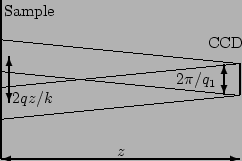
For the scattering from a thin sample, the intensities of the beams scattered at two symmetric angles are equal, and the phases are defined. Since the angles are symmetric, the interference of the scattered beams with the much intense transmitted beam gives two interference patterns, sinusoidal modulations, with the same wavevector, and a given phase. Changing $z$, the two diffraction patterns change their phase; at some $z$ they sums, and at other values they cancel out. This is the origin of the oscillations in the transfer function of shadowgraph technique, defined in Eq. (3.37). If the condition of Eq. (3.60) is met, the phases of the beams scattered at symmetric directions is random: on average, the transfer function is constant.

The vanishing of the $\left <EE\right >$ terms can be obtained also by increasing the thickness of the sample. When we pass from the two dimensional, Raman Nath scattering to the three dimensional, Bragg scattering, the correlations between the two beams scattered at the symmetric angles by a given sinusoidal modulation are not preserved. In shadowgraph language, the transfer function oscillations are washed out by superposing many layers, at different $z$. The thickness of the sample $\delta z$ must meet the condition $\delta z>k/q_1^2$.

Hosted by www.Geocities.ws