Each scatterer of the sample generates a diffraction pattern
which, at least in its far field, becomes larger and larger linearly,
as the distance ![]() from the screen and the sample is made longer.
So, for
from the screen and the sample is made longer.
So, for ![]() longer than a given distance, many diffraction patterns
overlap: the Wick formulas should become valid. Unfortunately, the
considerations of the previous section cannot be applied directly,
since the area the diffraction pattern has not been already defined
in a quantitative way.
longer than a given distance, many diffraction patterns
overlap: the Wick formulas should become valid. Unfortunately, the
considerations of the previous section cannot be applied directly,
since the area the diffraction pattern has not been already defined
in a quantitative way.
Now we will prove the Wick formula for the case of Siegert relation, by using the formalism developed in the previous section.
From the results of the previous section, we can evaluate the
intensity correlation function of the sum of the patterns,
at a given ![]() :
:
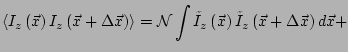 |
(3.51) | ||
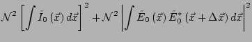 |
In order that Siegert relation holds, for a finite value of ![]() ,
we must impose that the term with the four point correlation
function is negligible compared to the two point ones:
,
we must impose that the term with the four point correlation
function is negligible compared to the two point ones:
![$\displaystyle \mathcal{N} \int{ \tilde{I}_z\left(\vec{x}\right) \tilde{I}_z\lef...
...ll \mathcal{N}^2 \left[\int{ \tilde{I}_0\left(\vec{x}\right) d\vec{x}}\right]^2$](img231.png) |
(3.52) |
![$\displaystyle \mathcal{N} \frac{ \displaystyle \left[\int{ \tilde{I}_z\left(\ve...
...t]^2 }{ \displaystyle \int{ \tilde{I}^2_z\left(\vec{x}\right) d\vec{x}} } \gg 1$](img232.png) |
(3.53) |
It should be noted that the validity of Vick formulas for a
given ![]() does not mean that the field is completely gaussian.
For example, we have shown that
does not mean that the field is completely gaussian.
For example, we have shown that
![]() for
for
![]() , where
, where
![]() is the intensity
correlation function of the diffraction pattern, defined as
is the intensity
correlation function of the diffraction pattern, defined as
![]() .
But this does not imply any uniform convergence. Its integral,
.
But this does not imply any uniform convergence. Its integral,
![]() ,
for example, is a constant, and does not vanishes as
,
for example, is a constant, and does not vanishes as
![]() .
This means that we can build suitable linear operators, acting on the field,
yelding
quantities which do not have a gaussian distribution.
A dramatic example can be obtained considering the scattering
from a two dimensional screen, with many holes of a given shape.
As
.
This means that we can build suitable linear operators, acting on the field,
yelding
quantities which do not have a gaussian distribution.
A dramatic example can be obtained considering the scattering
from a two dimensional screen, with many holes of a given shape.
As
![]() , the field meets the Vick formulas ever better.
But it is alwais possible to analyze an area, bigger than the
diffraction pattern of each hole, and to recover the shape
of the holes. This can be done by deconvolving the field by a
suitable function: it's the operation made by a lens, which creates
an image of the holes. The deconvolution gives any information
about the sample, including the fourth order correlations: the
deconvolved field is not gaussian. The gaussianity is only local:
once we defined an area, corresponding to the aperture of a lens,
there's a distance beyond which we are not able to recover the
shape of each hole, and so informations on higher order
correlation functions than second order ones are lost.
, the field meets the Vick formulas ever better.
But it is alwais possible to analyze an area, bigger than the
diffraction pattern of each hole, and to recover the shape
of the holes. This can be done by deconvolving the field by a
suitable function: it's the operation made by a lens, which creates
an image of the holes. The deconvolution gives any information
about the sample, including the fourth order correlations: the
deconvolved field is not gaussian. The gaussianity is only local:
once we defined an area, corresponding to the aperture of a lens,
there's a distance beyond which we are not able to recover the
shape of each hole, and so informations on higher order
correlation functions than second order ones are lost.
We can conclude that Eq. (3.55) implies only a local gaussianity; gaussianity is valid only when considering points inside an area small compered with the diffraction pattern of each scatterer. On the other hand, the knowledge of the field on a whole plane allows to recover any information on the correlation function of any order.