Gaussian field generated by the sum of many patterns.

Consider a monodisperse colloid, and the near field scattered light. The field can be decomposed into the sum of the waves coming from the different elements of the colloid. Thus at every distance from the colloid, the field will be given by the sum of many patterns, each randomly placed. An example of this is given in Fig. 3.4 and 3.5. Figure 3.4 shows the pattern: the intensity is linearily dependent on the field $f\left(\vec{x}\right)$, which we can consider given by the wave scattered by a particle of the colloid. Figure 3.5 shows the sum of the patterns, the function $\rho\left(\vec{x}\right)$:

$$\rho\left(\vec{x}\right)=\sum_{i=1}^N{f\left(\vec{x}-\vec{x}_i\right)}$$ (3.48)

where the $N$ $\vec{x}_i$ are randomly distributed in a surface of measure $S$.

Figure 3.4: Example of the field generated by a particle of the colloid.

Figure 3.5: Example of the field generated by many particles of the colloid.

Now we will evaluate the $P$-point correlation functions of the sum of many patterns, $\rho\left(\vec{x}\right)$. The results will be obteined, first, for fixed particle density $\mathcal{N}=N/S$, and $N\to \infty$; then we will show that, in a suitable limit, the $P$-point correlation functions, for $P\ge 4$, can be expressed in terms of two-point correlation function, corresponding to the Wick formula. In other words, every connected part of the correlation function developement vanishes: the field becomes gaussian. As a matter of fact, we will prove an extension of the well known central limit theorem.

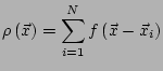
In the following, we will consider only functions with a vanishing average value, the other cases being easily obtained from this one. This simplifies the problem, since every odd-$P$-point correlation function will vanish.

The $P$-point correlation function of $\rho\left(\vec{x}\right)$ is:

$$\begin{multline} C\left(\Delta \vec{x}_2,\dots,\Delta \vec{x}_P\right)= \left<\r... ...\mathrm{d}\vec{x} \mathrm{d}\vec{x}_1 \dots \mathrm{d}\vec{x}_N } \end{multline}$$

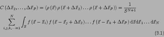
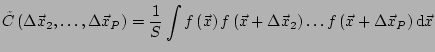
The value of the integral does not depend on all the values of the indices $i,j,k,\dots$, but only on which of them are equal; the sum involves $NP$ terms, but many of them are equal. For example, for $P=4$, the term with $i=1, j=2, k=3, l=4$ is equal to the one with $i=2, j=5, k=7, l=9$, but it is different from the one with $i=1, j=1, k=3, l=4$. The problem is thus to determine in how many ways we can obtain a given configuration.

The calculation can be made more easy using graphs. For evaluating a $P$-point correlation function, we draw $P$ points on a graph, each one corresponding to one of the points of the correlation function, $0, \Delta \vec{x}_2, \dots, \Delta \vec{x}_P$. Then, we group the points, so that every set contains an even number of points ^3.1. Each configuration corresponds to many values of the indices $i,j,k,\dots$; the number of them is the multiplicity of the graph. Every set corresponds to an operation of integration on a different $\vec{x}_i$. We call $G$ the number of sets; we will have only $G$ integration variables, being the integrand independent on the other $N+1-G$ variables. The integration on these variables gives a factor $S^{N+1-G}$. Moreover, every integration corresponds to the evaluation of the correlation function $\tilde{C}$ of the single pattern $f\left(\vec{x}\right)$:

$$\tilde{C}\left(\Delta \vec{x}_2,\dots,\Delta \vec{x}_P\right)= \f... ...vec{x}_2\right) \dots f\left(\vec{x}+\Delta \vec{x}_P\right) \mathrm{d}\vec{x}}$$ (3.49)

The multiplicity of the graph depends on $G$; its value is $N\left(N-1\right)\left(N-2\right)\dots\left(N-G+1\right)$. For $N\to \infty$, we can consider only the leading term $N^G$.

We can thus describe the rules for evaluating the correlation functions, as the sum of all the graphs. The value of every graph is the product of the factors given by each set. The factor is the product of $\mathcal{N}$ and the correlation function $\tilde{C}$, which correlates all the points in the set.

For example, we evaluate the two-point correlation function (Tab. 3.1) and the four-point correlation function (Tab. 3.2).

Table 3.1: Evaluation of the two-point correlation function.

$C\left(\Delta \vec{x}_1\right) = \mathcal{N} \tilde{C}\left(\Delta \vec{x}_1\right)$

Table 3.2: Evaluation of the four-point correlation function.

$C\left(\Delta \vec{x}_1,\Delta \vec{x}_2, \Delta \vec{x}_3\right) =$
	$\mathcal{N} \tilde{C}\left(\Delta \vec{x}_1,\Delta \vec{x}_2, \Delta \vec{x}_3\right)+$
	$\mathcal{N}^2 \tilde{C}\left(\Delta \vec{x}_1\right) \tilde{C}\left(\Delta \vec{x}_2-\Delta \vec{x}_3\right)+$
	$\mathcal{N}^2 \tilde{C}\left(\Delta \vec{x}_2\right) \tilde{C}\left(\Delta \vec{x}_1-\Delta \vec{x}_3\right)+$
	$\mathcal{N}^2 \tilde{C}\left(\Delta \vec{x}_3\right) \tilde{C}\left(\Delta \vec{x}_1-\Delta \vec{x}_3\right)$

For $\mathcal{N}\to \infty$, the leading term in the developement of the correlation function is the one with the higher power of $\mathcal N$: it is the one with the higher number of sets. Since sets with an odd number of elements have a vanishing contribution, the greatest number of sets can be obtained only by making sets of two points. This means that only two point correlation functions of the single pattern $\tilde{C}\left(\Delta \vec{x}\right)$ contribute to any correlation function $C\left(\Delta \vec{x}_1,\dots \right)$ of the sum.

Since $\mathcal{N}$ is dimensional, it is not possible to state if it is small or great. This means that we cannot define, in general, a value of $\mathcal{N}$ so great that the field becomes gaussian. The following heuristic considerations will show that the field is gaussian if $\mathcal{N}A\gg 1$, where $A$ is the area of one pattern, at least if we can define it in some ways. Consider a pattern $f\left(\vec{x}\right)=\alpha \chi_A\left(\vec{x}\right)$. The P-point correlation function of the pattern $f\left(\vec{x}\right)$, evaluated in $\Delta \vec{x}=0$, has the value $\tilde{C}\left(0,\dots\right)\alpha^PA$. Every graph will have a factor $\alpha^P$ and a factor $A^G$, where $G$ is the number of sets in the graph. So the factor $\mathcal{N}$ alwais appears multiplied by $A$. By imposing $\mathcal{N}A\gg 1$, we obtain that the only contributions to the correlation function of the sum of patterns comes from the two point correlation function of the single pattern: all the Wick formulas are valid. In order that $\mathcal{N}A\gg 1$, the mean number of scattering particles inside each area $A$ must be large: many pattern must overlap, in each point.

Hosted by www.Geocities.ws