Problems part 2 : System Modeling
and Analysis in the time domain
![]()
Problems
The Triangular Pulse as a Convolution
of Two Rectangular Pulses
The 2-sample wide triangular pulse ![]() can be expressed as a convolution of the one-sample rectangular
pulse with itself.
can be expressed as a convolution of the one-sample rectangular
pulse with itself.
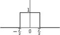
The one-sample rectangular pulse is shown above in
Fig and may be defined analytically as
where ![]() is
the Heaviside unit step function:
is
the Heaviside unit step function:
![$\displaystyle u(t) \isdef \left\{\begin{array}{ll}
1, & t\geq 0 \\ [5pt]
0, & t<0 \\
\end{array}\right..
$](index2_prob_files/image009.gif)
Convolving ![]() with
itself produces the two-sample triangular pulse
with
itself produces the two-sample triangular pulse ![]() :
:
While the result can be verified
algebraically by substituting ![]()
For ![]() .
.
Convolution of exponentials.
Cuthbert Nyack
|
As a simple example of
evaluating the convolution, consider the functions f1a(t)
and f2(t) shown in the diagrams
opposite. |
|
|
|
The general expression for
the convolution f(t) of two functions
with f2(t - t) shown opposite. f1(t) here corresponds to f1a(t) and f1a(t) is the same as f1a(t) with the variables changed. |
|
|
Because of the
discontinuity in f1a(t) then the
convolution fa(t) of f1a(t) and f2(t)
must be done in the 2 intervals of time t < 0 and t ³ 0. For t < 0, the convolution is zero and for t ³ 0 it is given by the expression below.
The diagram opposite shows f1a(t) in red f2(t)
in blue and fa(t) in purple.
|
|
|
The calculation of the
convolution can be extended by considering the pulse opposite instead of a
step. Here there are 2 discontinuities and the convolution must be evaluated
in 3 intervals. |
|
|
For t > 1 the convolution of f1b(t)
and f2(t) is given by fb(t) in the equation below.
The limits of the
integration are 0 and 1 since the interval from 0 to 1 is the only one where
both f1b(t)
and f2(t - t)
are nonzero. |
|
|
The final result for the
convolution f(t) is now given by:- |
|
|
In the diagram opposite the
function f1b(t) is extended to f1c(t) by adding a step for t ³ 2. |
|
|
For t ³ 2, the convolution of f1c(t)
and f2(t) is given by fc(t) in the expression below. The
integral must be evaluated over the 2 intervals 0 to 1 and 2 to t for which
both functions are nonzero.
|
|
|
The final result for the
convolution f(t) is now given by:- |
|
|
A modified version of f1b(t) is shown in the diagram opposite
as f1d(t). Instead of the pulse
dropping to zero at t = 1, it follows a ramp with slope -1 to reach 0 at t =
2. For t up to 1 the convolution of f1d(t)
and f2(t) is the same as f1b(t) and f2(t)
but differs for larger values of t. |
|
|
In the interval 1 £ t £ 2 the convolution of f1d(t)
and f2(t) is given by fd(t) shown opposite. |
|
|
And for the interval t ³ 2 the convolution of f1d(t)
and f2(t) given by fe(t)
shown opposite. |
|
|
The final result for the
convolution f(t) of f1d(t)
and f2(t) is now given by:- |
|
Go to first part : Principles of Signal and Systems Modeling Concepts
Go to second part : System Modeling and Analysis in the time domain