Part 1: Signal and System Modeling Concepts :

1-1) This part focus with systems and the interaction of signal in systems . But what is a system according with the Institute of Electrical and Electronic

Engineer dictionary defines a systems as “an integrated whole even though composed of diverse , interacting structures or sub junctions” in few words is a

combination and interconnection of several components to perform a desired task. We will focus our attention to linear systems because most of the engineering

aspects are closely approximated by linear systems and exist many techniques for analyzing them.

A signal may be considered to be a function of time that represents a physical variable of interest associated with a system . In electrical systems , signals usually represent

currents and voltages , whereas in mechanical systems , they represent forces and velocities.

1-2) Signals Models:

Deterministic Signals : A deterministic signal can be modeled as completely specified functions of time .

Example: x(t)= At²+Bt -∞ < t < ∞ . (1-1)

Where A and B are constants shown in the following figure (1-1) .

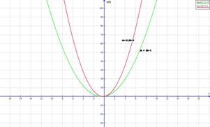
Fig 1-1

(a) Signal of equation 1.

An example of a deterministic signal that is not continuous function of time is the unit pulse , denoted as ∏ (t) and defined as

(1-2 )

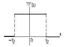Fig 1-2 Unit pulse signal

2) Periodic and Aperiodic signals

A signal x(t) is periodic if only if :

x(t+T₀)= x(t) -∞ < t < ∞ . (1-3)

where the constant T₀is the period . The smallest value of To such that (1-3) is satisfied is referred to as the fundamental period simply referred as a period .

Any deterministic signal satisfying (1-3) is called aperiodic.

An example of a periodic signal is a sinusoidal signal:

-∞ < t < ∞ (1-4)

Where A is the amplitude , is the frequency in hertz and the angle of phase.

We know that where is the frequency in rad/seg.

The Period of this signal is : which can be verified by direct substitution in equation (1-3) .

From equation (1-4) we have:

………. (1-5)

But cos(2) =1 and sin(2)=0 in equation (1-5) we have :

since and thus the equation (1-3) is satisfied.

The sum of two or more sinusoids may or may not be periodic , depending on the relationships between their respective periods or frequencies .

If and are the frequencies of two sinusoids where n and m are integers : is called the fundamental frequency , thus their

corresponding periods and are related by .

Fig. 1-3 Graph of a sinusoidal

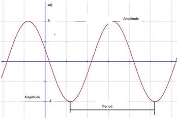Signal

3) Phasor Signals and Spectra

When we are working with signals it is convenient to represent real signals in terms of complex quantities that is why we use phasors , according

phasors theory a signal can be represented by :

…….(1-6)

For a sinusoidal signal we can represent the real part (Re(…)) by:

-∞ < t < ∞ (1-7)

The complex signal is:

-∞ < t < ∞ (1-8)

This rotating phasor signal have three parameters : A the amplitude , the phase . and >0 the radian frequency .

Another important expression is the Euler’s which a complex variable can be represented in terms of sin and cos.

…………………………(1-9)

…………………………(1-10) thus

…………………………(1-11)

…………………………(1-12)

A sinusoidal function can be represented using equation (1-11)

, -∞ < t < ∞ (1-13)

Which is a representation in terms of complex conjugate quantities.

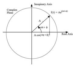Fig. 1-4 Phasor representation of a wave

We can plot the amplitude and phase in two ways.

Single-sided amplitude and phase spectrum is used because these spectral plots have points or lines only for positive frequencies.

Double-sided amplitude and phase spectrum is used at and positive and negative frequencies , it is necessary to note that double-sided

spectra the lines at negative frequencies are present because is necessary to add complex conjugate phasors , Amplitude spectrum has even symmetry about

the origin and the phase spectrum has odd symmetry about the origin.

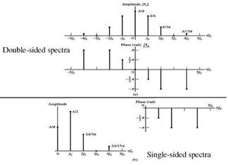
Fig. 1-5 Amplitude and phase spectra

4) Singularity Functions

This aperiodic signals play an important role in the communication systems .We begin by showing the unit step and unit ramp and using them to represent

more complicated functions .

Unit step function (Heaviside function ) is defined as :

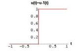
…………………………(1-14)

Fig 1-6 Unit step function

The value of at t=0 will not be specified at this time (next we will show that u(0)=1/2 ) Other singularity functions are defined in terms of

by the relation

i=……,-2,-1,0,1,2……. (1-15)

Taking first derivative to equation (1-15) we can represent as:

……………………. (1-16)

Unit ramp function using equation (1-15) in the unit step function we have

(1-17)

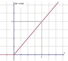
Fig 1-7 Unit ramp function

Unit parabolic function using equation (1-15) in the unit ramp function we have

……………………….. (1-18)

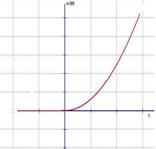
Fig 1-8 Unit parabolic function

We can shift any signal in the time axis , if we replace by if >0 the signal is shifted to the right , if <0 the signal is shifted to the left .

Using in the unit step function with =1/2 we have:

……………………. (1-19a)

……………….......... (1-19b)

Using equation 1-19 we can represent unit pulse function

(1-20)

Another important function is the unit impulse function or delta function.

Unit impulse function or delta function which has the following properties :

…………………………..(1-21a)

And

……………………………………(1-21b)

From equation 1-21b we can state that the area of the delta function is unity.

We have a mathematical definition of the unit impulse function proceeds by defining in terms of the functional :

……………………………………(1-22)

Where is continuous at .

has the following properties:

……………………………………(1-23)

Using the equation 1-23 with a=-1 we can see that : that is an even function.

Another property of the delta function is the sifting property :

……………………………………(1-24)

is continuous at , if we change in the equation 1-24

We have :

……………………………………(1-25)

An alternative form of the equation 1-22 is :

……………………………………(1-25)

Equation 1-26 is known as a convolution integral.

If we have integrals with finite limits moreover defining to be zero outside a certain interval , thus :

………….…………………(1-26)

Another properties of delta function are:

…………………………………(1-27)

…………………………(1-28)

In general if the nth derivative of exists and continuous at it can be represented by :

………………(1-29)

Now that we know delta function we may represent unit step function in terms of delta function.

………………(1-30)

Or taking first derivative to equation (1-30) we can represent as:

………………(1-31)

5) Energy and Power Signals

There are three classifications of signals according to study of energy and power . Those having finite energy , those having finite average power and

signals that satisfy neither .

Suppose that is the voltage across a resistance producing a current , thus the instantaneous power per ohm is :