
Part 2: System Modeling and analysis in the time domain.
In the first part we discussed some continuous-time signal models , in this part we will discuss some techniques in time domain.
There are several mathematical procedures for systems in time domain , but we will focus on linear time invariant systems.
We begin our study analyzing the convolution integral which is a powerful tool for analysis of linear , time – invariant systems.
Representation of systems
There are a representation
between input ![]() and
output
and
output ![]() variables of a system
variables of a system

![]()
![]()

The dependence between input and output variables is related for the following
![]()
Convolution integral
The convolution integral has the following form :
![]()
The Evaluation of the Convolution Integral
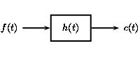
Consider the system described by the differential equation:
![]()
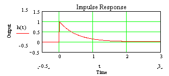
which has an impulse response given by
![]()
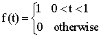
We will use convolution to find the zero input response of this system to the input given by
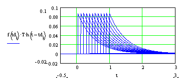
Convolution as sum of
impulse responses
|
For continuity with the page deriving the convolution integral we can approximate the input by a series of impulses... |
|
|
plot the response of the system to each of these impulses... |
|
|
and plot the response as the sum of the individual responses
|
|
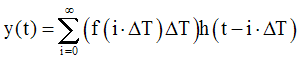
Convolution Integral
Likewise the convolution can be considered from the point of view of the convolution integral.
![]()
.
The Mechanics of Using the Convolution Integral
To find the output of the system with impulse response
![]()
to the input
we will use the convolution integral
![]()
Because the input function has three distinct regions t<0, 0<t<1 and 1<t, we will need to split up the integral into three parts.
Part 1: t<0
For t<0 the argument of the impulse function (t-t) is always negative. Since h(t-t)=0 for (t-t)<0, the result of the integral is zero for t<0.
This situation is depicted graphically below (t=-0.2):
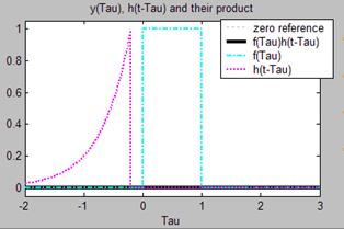
So the result for the first part of our solution is
![]()
Part 2: 0<t<1
For 0<t<1 we need to evaluate the integral only from t=0 to t=t, since f(t)=0 when t<0, and h(t-t)=0 when (t-t)<0 (or, equivalently t<t). So the integral becomes, in effect:
![]()
This situation is depicted graphically below (t=0.5):
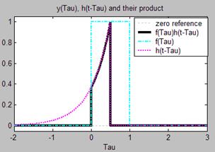
We can now evaluate the integral of the solid black line:
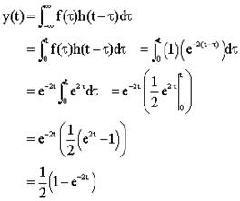
Thus, the result for the second part of the solution is
![]()
Part 3: 1<t
For 1<t we need to evaluate the integral only from t=0 to t=1, since f(t)=0 when t<0 and when t>1. So the integral becomes, in effect:
![]()
This situation is depicted graphically below (t=1.2):
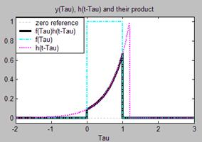
We can now evaluate the integral:
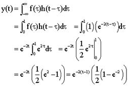
Thus, the result for the third part of the solution is:
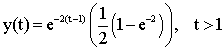
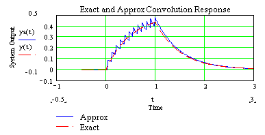
The complete answer.
We can get the results for all time by combining the solutions from the three parts.
![]()
![]()
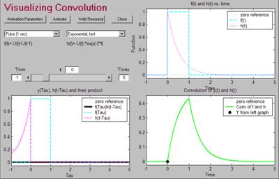
This result is shown below. Click on the image to see an animation of the convolution operation.
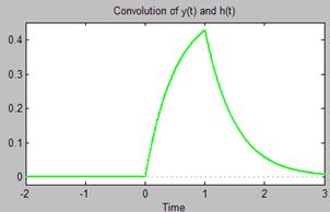
The convolution integral is a completely general method for finding the output of a linear system for any input.
|
Convolution properties |
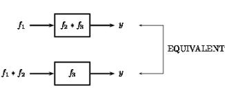
Associativity
theorem 1: Associative Law
f1(t) *(f2(t) *f3(t)) =(f1(t) *f2(t)) *f3(t)
|
Figure 1: Graphical implication of the associative property of convolution. |
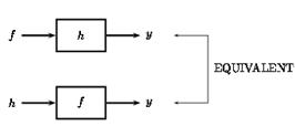
Commutativity
theorem 2: Commutative Law
|
y(t) |
= |
f(t) *h(t) |
|
y(t) |
= |
h(t) *f(t) |
Proof
To prove this equation all we need to do is make a simple change of variables in our convolution integral (or sum),
y(t) =∫−∞∞f(τ) h(t−τ) dτ
By letting τ=t−τ , we can easily show that convolution is commutative:
|
y(t) |
= |
∫−∞∞f(t−τ) h(τ) dτ |
|
y(t) |
= |
∫−∞∞h(τ) f(t−τ) dτ |
f(t) *h(t) =h(t) *f(t)
|
Figure 2: The figure shows that either function can be regarded as the system's input while the other is the impulse response. |
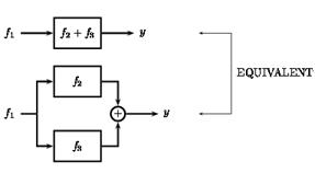
Distribution
theorem 3: Distributive
Law
f1(t) *(f2(t) +f3(t)) =f1(t) *f2(t) +f1(t) *f3(t)
Proof
The proof of this theorem can be taken directly from the definition of convolution and by using the linearity of the integral.
|
Figure 3 |
Time
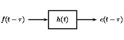
Shift
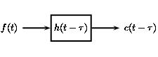
theorem 4: Shift Property
For c(t) =f(t) *h(t) , then
c(t−T) =f(t−T) *h(t)
and
c(t−T) =f(t) *h(t−T)
|
Subfigure 1
Subfigure 2
Subfigure 3 Graphical demonstration of the shift property. |
Convolution
with an Impulse
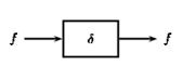
theorem 5: Convolving with Unit Impulse
f(t) *δ(t) =f(t)
Proof
For this proof, we will let δ(t) be the unit impulse located at the origin. Using the definition of convolution we start with the convolution integral
f(t) *δ(t) =∫−∞∞δ(τ) f(t−τ) dτ
From the definition of the unit impulse, we know that δ(τ) =0 whenever τ≠0. We use this fact to reduce the above equation to the following:
|
f(t) *δ(t) |
= |
∫−∞∞δ(τ) f(t) dτ |
|
f(t) *δ(t) |
= |
f(t) ∫−∞∞(δ(τ)) dτ |
The integral of δ(τ) will only have a value when τ=0 (from the definition of the unit impulse), therefore its integral will equal one. Thus we can simplify the equation to our theorem:
f(t) *δ(t) =f(t)
|
Subfigure 1
Subfigure 2 Figure 1: The figures, and equation above, reveal the identity function of the unit impulse. |

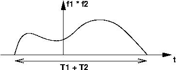
Width
In continuous time, if Duration(f1) =T1 and Duration(f2) =T2 , then
Duration(f1*f2) =T1+T2
|
Subfigure 1
Subfigure 2
Subfigure 3 Figure 1: In continuous-time, the duration of the convolution result equals the sum of the lengths of each of the two signals that are convolved. |
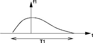
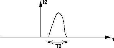
In discrete time, if Duration(f1) =N1 and Duration(f2) =N2 , then
Duration(f1*f2) =N1+N2−1
Causality
If f and h are both causal, then f*h is also causal.
Go to problems for second part
Go to first part : Principles of Signal and Systems Modeling Concepts
Go to third part : The Fourier series
Go to fourth part : Laplace Transform