| The Hamiltonian Path Problem and the DNA solution to it |
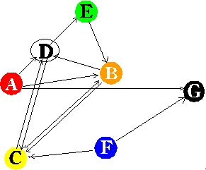
| The Problem Figure 1 shows a diagram of the Hamiltonian Path problem. The objective is to find a path from start to end going through all the points only once. This problem is difficult for conventional computers to solve because it is a non-deterministic polynomial time problem NP). NP problems are intractable with deterministic (conventional/serial) computers, but can be solved using non-deterministic (massively parallel) computers. A DNA computer is a type of non-deterministic computer. The Hamiltonian Path problem was chosen because it is known as NP-complete; every NP problem can be reduced to a Hamiltonian Path problem |
| Figure 1: The Hamiltonian Path problem. The goal is to find a path from the start city to the end city going through every city only once. |
| Solving the Problem |
| The following algorithm solves the Hamiltonian Path problem Generate random paths that begin with start city (A) and conclude with end city (G). If the graph has 'n" cities, keep only those paths with n cities. (n=7). Keep only those paths that enter all cities at least once Any remaining paths are solutions |
| The key to solving the problem was using DNA to perform the five steps in the above algorithm. The following operations can be performed with DNA Synthesis of a desired strand Separation of strands by length Merging -mix the strands to perform hybridisation Extraction- extract strands containing a given pattern Melting /Annealing- break/bond two single stranded DNA molecules with complementary sequences Amplification- Make multiple copies of DNA strands using PCR Cutting- Cut at specific sites using restriction enzymes Ligation- Ligate DNA strands with the complementary sticky ends using ligase Detection- Conform the presence /absence of DNA in a given test tube- (By gel electrophoresis) The above operations may be used to program a DNA computer |
| Programming with DNA |
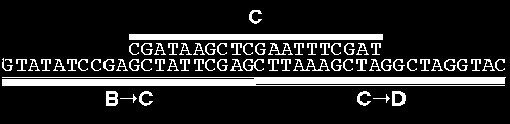
| To implement step 1 of the algorithm, Adleman created a 20-mer sequence of DNA for each city Athrough G. For each path i>j, an oligonucleotide was created that was the 3' 10-mer of i and 5' 10-mer of j (see figure 2). A>B contained all of A and the 5' 10-mer of B, and E G contained the 3' 10-mer of E and all of G to eliminate any possible sticky ends. For each city i, a Watson-Crick complementary oligonucleotide was synthesized and designated ~i. |
| For each city except A and G, and for each path, 50 pmol of and 50 pmol of i>j, respectively, were mixed together in a single ligation reaction. The oligonucleotides served as splints to bring paths between common cities to associate for ligation. The ligation reaction therefore resulted in the formation of DNA molecules encoding random paths through the graph. |
| Figure 2: Encoding a path in DNA. For each city A through G, a random 20-mer oligonucleotide was generated. A complementary sequence was generated for each city: ~C is the oligonucleotide complementary to the oligonucleotide C, which represents city C. For each path, a 20-mer oligonucleotide was created which was the 3' 10-mer of the originating city, and the 5' 10-mer of the target city, except for paths from A or to G. Shown above is DNA encoding the path from B>C>D. |
| Step 2 was implemented by using A and ~G as primers for PCR to amplify all "paths" from starting with A and ending with G. |
| For step 3, the product of step 2 was run on an agarose gel, and the 140 bp band (corresponding to a dsDNA path entering exactly seven cities) was excised and soaked in double-distilled H2O to extract the DNA. This product was then PCR amplified and gel-purified several times to enhance its purity. |
| In order to complete step 4, the product of step 3 was affinity-purified with a biotin-avidin magnetic beads system. The dsDNA from step 3 was melted and the ssDNA product was incubated with ~A conjugated to magnetic beads. Only those ssDNA molecules that entered city A at least once were annealed to the bound ~B and retained. The process was successively repeated with ~C, ~D, ~E, and ~F. |
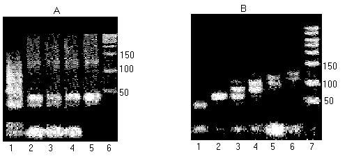
| Step 5 was performed by amplifying the product of step 4 with PCR and running it on a gel. Figure 3 shows the results of these procedures. In figure 3A, lane 1 is the result of the ligation reaction in step 1. The smear is consistent with the construction of molecules encoding random paths through the graph. Lanes 2-5 show the results of the PCR reaction in step 2. The densest bands correspond to the amplification of molecules encoding paths that began at A and ended at F. |
| Figure 3B shows graduated PCR of the final product of the computer. Graduated PCR allows one to "print" the results of a computation, using A as the right primer and ~B through ~G as the left primer lanes 1-7, respectively. The graduation shows the progression from A>B>C>D>E>F>G. |
| The above procedure took approximately one week to perform. Although this particular problem could be solved on a piece of paper in under an hour, when the number of cities is increased to 70, the problem becomes too complex for even a supercomputer. The fastest supercomputers can currently perform 1000 million instructions per second (MIPS); a single DNA molecule requires approximately 1000 seconds to perform an instruction (.001 MIPS). Obviously of you want to perform one calculation at a time (serial logic), DNA computers are not a viable option. However, if one wanted to perform many calculations simultaneously (parallel logic), a computer such as the one described above can easily perform 10^14 MIPS. DNA computers also require less energy and space. While existing supercomputers operate 10^9 operations per Joule, a DNA computer could perform 2 x 10^19 operations per Joule (10^10 times more efficient). Data can be stored on DNA at a density of approximately 1 bit per cubic nm, while existing storage media require 10^12 cubic nm to store 1 bit. |
| Figure 3 Agarose gel electrophoresis of various products of Adleman's DNA computer. (A) Raw product of the ligation reaction in lane 1; lanes 2-5 contain the PCR amplification of the product of the ligation reaction; lane 6 contains the molecular weight marker in base pairs. (B) Graduated PCR of the final product of the experiment revealing the Hamiltonian Path in lanes 1-6; molecular weight marker in lane 7. |
 |
| Adleman's DNA Computer In 1994, Leonard Adleman took a giant step towards a different kind of chemical or artificial biochemical computer. He used fragments of DNA to compute the solution to a complex graph theory problem. Adleman's method utilized sequences of DNA's molecular subunits to represent vertices of a network or `graph.. Thus, combinations of these sequences formed randomly by the massively parallel action of biochemical reactions in test tubes described random paths through the graph. Using the tools of biochemistry, Adleman was able to extract the correct answer to the graph theory problem out of the many random paths represented by the product DNA strands. Like a computer with more than one processor, this type of DNA computer is able to consider many solutions to a problem simultaneously. Moreover, the DNA strands employed in such a calculation (approximately 10^23) are many orders of magnitude greater in number and more densely packed than the processors in today's most massively parallel electronic supercomputer. |
| THE FIRST EVER DNA COMPUTER WAS IN A TEST TUBE |
| FFD |
| FFD |
 |
 |