Next: Pulse stabilization
Up: Limits of ultrashort pulse
Previous: Limits of ultrashort pulse
Nature of the stability boundaries
The
 decreases as a result of the
 increase. Such behavior can be obtained also on the basis of the
soliton model. For example, in the weak-nonlinear limit one can
obtain the following condition of the background amplification
[2]:
increase. Such behavior can be obtained also on the basis of the
soliton model. For example, in the weak-nonlinear limit one can
obtain the following condition of the background amplification
[2]:
(curve 2 in Fig.
![[*]](crossref.gif) ). Here we keep the
normalization of
). Here we keep the
normalization of
 and
and
 to
to
 and
and
 ,
respectively. We have only qualitative agreement with the
numerical results owing to the weak-nonlinear approximation and
the simplified model of the gain behavior in the referenced model.
However even this simplified model agrees with numerical
calculation for the lower stability threshold by the order of
magnitude.
As it can be seen from the Fig.
, the behavior of the
lower stability boundary in the region of positive GDD agrees with
our qualitative treatment as well. We have to stress that the
destabilization in the framework of the soliton model takes place
only for the chirped pulses, while it is not a necessary condition
in the numerical model in the region of negative GDD. The curve 1
in Fig.
shows the location of the system parameters
corresponding to the chirp-free sech-pulse for the
weak-nonlinear approximation (this is
,
respectively. We have only qualitative agreement with the
numerical results owing to the weak-nonlinear approximation and
the simplified model of the gain behavior in the referenced model.
However even this simplified model agrees with numerical
calculation for the lower stability threshold by the order of
magnitude.
As it can be seen from the Fig.
, the behavior of the
lower stability boundary in the region of positive GDD agrees with
our qualitative treatment as well. We have to stress that the
destabilization in the framework of the soliton model takes place
only for the chirped pulses, while it is not a necessary condition
in the numerical model in the region of negative GDD. The curve 1
in Fig.
shows the location of the system parameters
corresponding to the chirp-free sech-pulse for the
weak-nonlinear approximation (this is
 [17]; we keep the usual normalizations). The
vicinity of the stability boundary to this curve causes the
destabilization of the nearly chirp-free pulse.
The agreement with the soliton model results from the
comparatively small loss saturation for small
. The
strong deviation from the weak-nonlinear model takes place for
[17]; we keep the usual normalizations). The
vicinity of the stability boundary to this curve causes the
destabilization of the nearly chirp-free pulse.
The agreement with the soliton model results from the
comparatively small loss saturation for small
. The
strong deviation from the weak-nonlinear model takes place for
 , where the pulse intensities are
sufficiently large for the strong loss saturation.
The referenced expression for
explains also
the increase of the stability boundary as a result of the
modulation depth decrease (see lower boundary of the A region
for
, where the pulse intensities are
sufficiently large for the strong loss saturation.
The referenced expression for
explains also
the increase of the stability boundary as a result of the
modulation depth decrease (see lower boundary of the A region
for
 0 in Fig.
, b) and the weak
dependence of the lower stability boundary on other laser
parameters (with the exception of
0 in Fig.
, b) and the weak
dependence of the lower stability boundary on other laser
parameters (with the exception of
 ) for the large
values of
(see Figs.
, c, e, f).
Formally, the dependence of
on
) for the large
values of
(see Figs.
, c, e, f).
Formally, the dependence of
on
 is obvious in the weak-nonlinear approximation: the expansion of
Eq. () on
is obvious in the weak-nonlinear approximation: the expansion of
Eq. () on
 gives
gives
 as the
self-amplitude modulation coefficient in the first order. The
decrease reduces the contribution of the self-amplitude
modulation, i. e. the difference between the pulse and background
net-gain, thus favoring the pulse destabilization.
The influence of the self-phase modulation on the pulse stability
can be interpreted in the following way. Increasing
favors the pulse destabilization because the pulse energy
decreases with growing spectral loss as a result of the pulse
spectrum expansion. Additionally, this spectral expansion reduces
the gain saturation (
as the
self-amplitude modulation coefficient in the first order. The
decrease reduces the contribution of the self-amplitude
modulation, i. e. the difference between the pulse and background
net-gain, thus favoring the pulse destabilization.
The influence of the self-phase modulation on the pulse stability
can be interpreted in the following way. Increasing
favors the pulse destabilization because the pulse energy
decreases with growing spectral loss as a result of the pulse
spectrum expansion. Additionally, this spectral expansion reduces
the gain saturation (
 ). This also
leads to the pulse destabilization by the background. The
growth intensifies the gain saturation and so
stabilizes the pulse against the background amplification (Fig.
, d). Here we do not consider the possible
stabilization against automodulations produced by the self-phase
modulation [17].
The contribution of the destabilization due to the bounded
perturbation growth complicates the picture. Since the amplitude
of such perturbation scales with the pulse energy [42],
[44], the decrease of the pulse energy will result in
the pulse stabilization against this instability. The pulse energy
decreases for
). This also
leads to the pulse destabilization by the background. The
growth intensifies the gain saturation and so
stabilizes the pulse against the background amplification (Fig.
, d). Here we do not consider the possible
stabilization against automodulations produced by the self-phase
modulation [17].
The contribution of the destabilization due to the bounded
perturbation growth complicates the picture. Since the amplitude
of such perturbation scales with the pulse energy [42],
[44], the decrease of the pulse energy will result in
the pulse stabilization against this instability. The pulse energy
decreases for
 , but increases with
. Hence the
, but increases with
. Hence the
 defining the pulse
destabilization increases due to the
increase (see
Figs.
). For some
defining the pulse
destabilization increases due to the
increase (see
Figs.
). For some
 switching between
destabilization mechanisms is possible (see the transition from
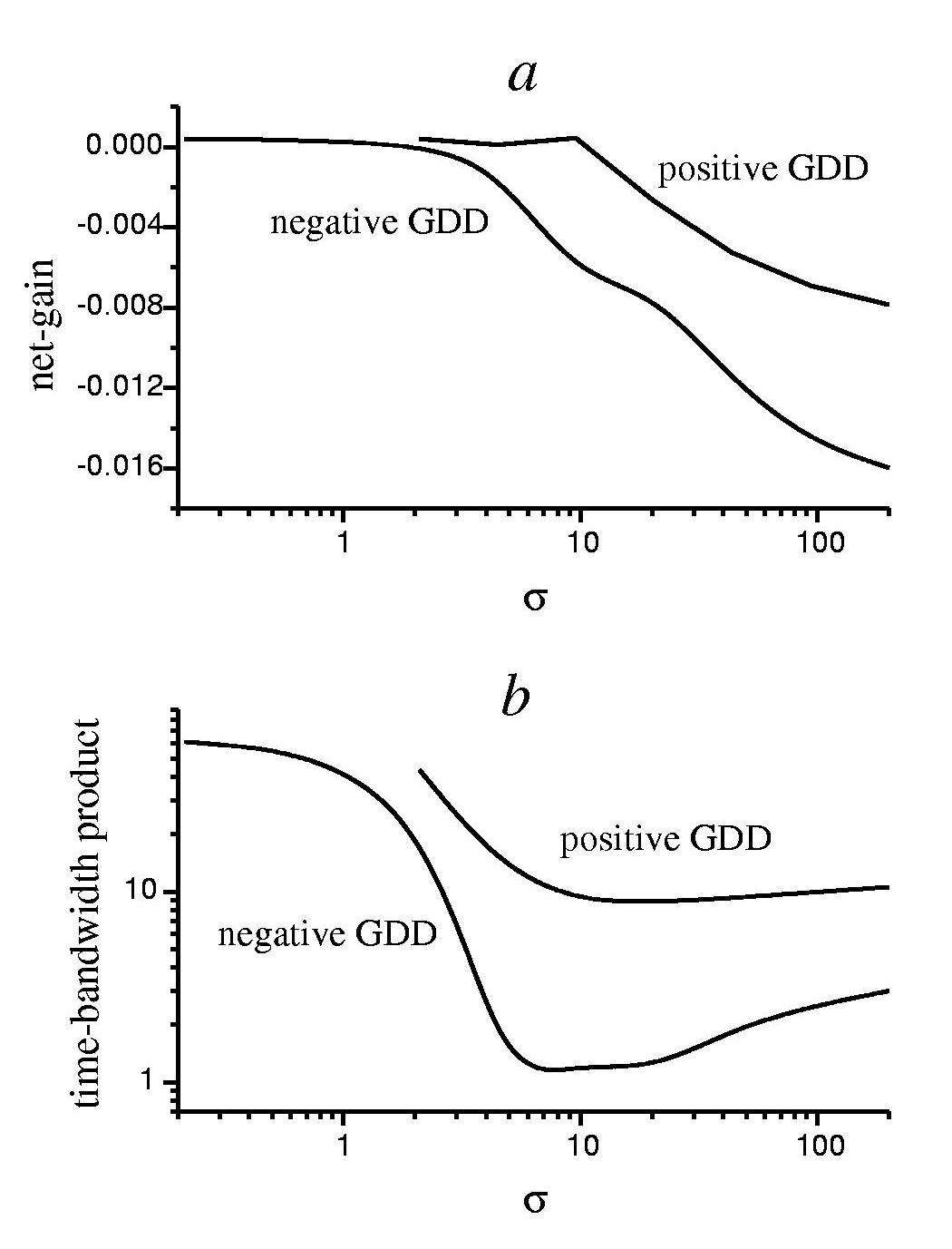
the positive to the negative net-gain and from the chirped to
chirp-free pulses at the stability boundary presented in Fig.
). Since the pulse duration decreases with
decrease, such switching (if it takes place) confines the
minimal duration of the ultrashort pulses (the minimal pulse
widths are shown by points in Figs.
). It should be
noted that destabilization due to the spectral loss can occur also
due to the chirp growth. This is illustrated by the Fig.
, b, where the pulse spectral width at the
stability boundary is shown to be as much as 50 times that of the
bandwidth-limited pulse.
switching between
destabilization mechanisms is possible (see the transition from
the positive to the negative net-gain and from the chirped to
chirp-free pulses at the stability boundary presented in Fig.
). Since the pulse duration decreases with
decrease, such switching (if it takes place) confines the
minimal duration of the ultrashort pulses (the minimal pulse
widths are shown by points in Figs.
). It should be
noted that destabilization due to the spectral loss can occur also
due to the chirp growth. This is illustrated by the Fig.
, b, where the pulse spectral width at the
stability boundary is shown to be as much as 50 times that of the
bandwidth-limited pulse.
Figure:
The net-gain (a) and
time-bandwidth product related to the Schrödinger soliton one
(b) at the single-pulse stability boundary shown in Fig.
, a.
|
|
Thus, the existence of the minimal and maximal
defining
the pulse stability results from the two different mechanisms of
the ultrashort pulse destabilization, viz., the destabilization
due to the continuum growth and pulse splitting due to the
increase of the bounded perturbations. The twofold character of
the destabilization complicates the laser optimization, as
considered in the next section.
Next: Pulse stabilization
Up: Limits of ultrashort pulse
Previous: Limits of ultrashort pulse
V.L. Kalashnikov
2002-12-28