MICROSOFT EXCEL 2000
Copyright CIT, 1999-2000. All rights reserved.

BÖLÜM 2. BASİT BİR HESAPLAMA SAYFASININ OLUŞTURULMASI/2

Sayıların girilmesi
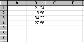
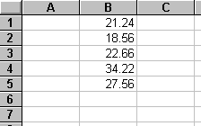
Amerikalı bir arkadaşınız evinizde misafir olarak bir hafta kalacak. Arkadaşınız Amerikadaki eşine hergün telefon ediyor. Konuşmaları günlere göre şu şekildedir: Pazartesi günü 21.24$, Salı 18.56$, Perşembe 4.22$ ve Cuma günü için 27.56$ lık konuşmalar yapmıştır.

Adım 2.8 Yukarıdaki verileri aşağıdaki gibi giriniz

Şekil 2.6

Bir dakika Çarşamba günü yapılan konuşma unutulmamalıdır. B3 hücresine Çarşamba günü yapılan konuşma tutarı eklenmelidir. Bunun için B3 hücresi ve altındakiler aşağı bir hücre kaydırılmalıdır. Çarşamba gününün tutarı oş hücreye yazılmalıdır.

Adım 2.9 3 üncü satırı tıklayınız. Bu satır aşağıdaki gibi gösterilecektir.

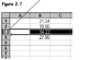
Şekil 2.7

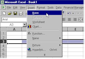
Adım 2.10 Seçenekler listesinden Ekle ve Satır ı seçiniz.

Şekil 2.8

Hesaplama sayfası aşağıdaki şekildeki gibi olacaktır.

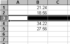
Şekil 2.9

Adım 2.11 B3 hücresine 22.66 değerini giriniz.

Şekil 2.10

Bu yöntemi sütun eklemek için yapabilirsiniz.

Bir satırı silmek için Edit menüsünden Sil seçeneğinden yararlanabilirsiniz. Klavyeden silme ile menüden silme arasındaki farka dikkat ediniz.

Adım 2.12 B1 den B5 e kadar olan hücreleri seçip daha sonra siliniz ve içeriği boş bir hesaplama sayfası oluşturunuz.

Hesaplamalar
There is obviously not much point in setting up numbers if you are not going to do anything with them. What we shall do now is see how Excel enters equations.

Aşağıdaki örnekleri dikkat ediniz

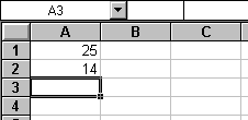
Şekil 2.11

Adım 2.13 Click on cell A1 and enter the value 25. Enter the value 14 into cell A2.

In cell A3 we want to put the sum of 25 and 14, but we do not write =25+14 (which is valid). What we really want to say is add the value stored in cell A1 to the value stored in cell A2 and store the result in A3.

Step 2.14 Click on cell A3 to make sure it is selected.

Step 2.15 Enter the following equation =A1+A2

This will total the contents of cells A1 and A2 and store the result in A3. Don’t forget the = sign which tells Excel that it is an equation.

Your spreadsheet should now look as follows

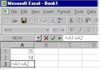
Figure 2.12

Note the equation is printed in the formula bar.

Step 2.16 Click on the Enter button.

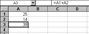
Şekil 2.13

Note how the equation appears in the formula bar, but the result appears in A3. To emphasise why we enter =A1+A2 rather than =25+14

Adım 2.17 Change the value in A1 to 26. The spreadsheet should look as follows

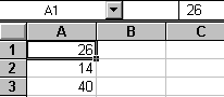
Şekil 2.14

See that A3 has changed as well, because the equation tells Excel to add the contents of A1 and A2 together, not 25 and 14.

Exercise two
Enter the values 25 and 15 into cells B2 and B3, and their sum in B4.

Exercise three
Enter values 18.2, 17.4, 5.2 into cells A2, B2 and C2 and their sum in D2. Did you forget the = sign at the beginning of equation?

Subtraction
To find the difference between the values in two cells write

=A1-A2

Multiplication
To find the product of the values in 2 cells write

=A1*A2

Notice the multiplication symbol used is the asterisk *.

Bölüm
To find the ratio of the values in 2 cells write

=A1/A2

Alıştırma 4
Work out what should be calculated for the following equations

Şekil 2.15

Hesaplama sayfasını cevaplarınızla kontrol ediniz.

Home | Other Courses | Notes | Feedback