Departmental Processing
Turnaround Estimation Project
Home
Problem definition
Data collected
Regression model
Analysis
Stepwise
Final model
Forecast Model for Duration
Recommendation
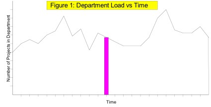
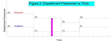
Load Chart