Motor Vehicle Emission Modeling near Highways and Arterial Streets

Motor Vehicle Emission Modeler and Analyzer (Lines 1.0)

Multiple Source Air Quality Modeler/Analyzer

Quasi-3D Refined Flow/ Contaminant Transport Modeling(CFD)

Uses:

Air quality analysis and evaluation for the effects of exhaust gas emission from motor vehicles in urban and rural zones.

Teaching software for courses relative to ambient air quality modeling and pollutant transport process.

* Versatile multi-line source dispersion software; model based on revised famous codes in the world (CALINE3, CAL3QHC) with easy-to-use GUI, self-contained map support tool, results' visualization and analysis kit as well as help system used in various Windows-based microcomputers.

* User-friendly powerful map support tool for pre- and pro-processing, including map basic color inspection, map-scale determination, road orientation, geometrical date auto-inserter to tables, receptor dispose, digital map background, map enlargement, shrink, storage and printing,....

* Up-to-date calculated results' visualizations, including 3 types of 2D contouring (homochromatic and color contour lines, color filled image), 2 methods for setting values of contour lines, displaying labeled coordinate axes with titles and ticks, selections of plotting grid lines, borders, vane and marked receptors. By using mouse, buttons and a few of keys, users can easily obtain various graphics.

* self-supplied results' analyzers both for displaying point coordinates and model-calculated concentration, and maximum, minimum and mean concentrations of local area (see Ex-5, Figure 1 and corresponding instruction).

* Convenient data input through dialog boxes, tables and digital map; input data display, revision, printing and storage; output results' display, print and storage.

* Easily simulating and analyzing concentration fields of inert pollutants (CO, suspended particulates ...), caused by traffic transportation in urban and rural zones as well as in small scale regions near highways and arterial streets.

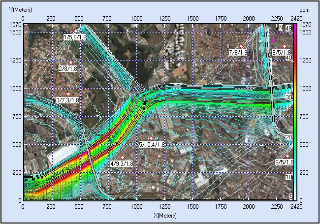
Motor Vehicle Emission Modeler and Analyzer (Lines 1.0, Lines 2.0) are versatile dispersion models with the support of Graphical User Interface (GUI) and Map Information Tool for simulating and predicting the concentrations of inert pollutants produced by traffic transportation, such as carbon monoxide(CO), particulates, and so on, in urban and rural zones as well as small-scale regions near highways and arterial streets. The Models, bases on the Gaussian diffusion equation, were originally developed by CALINE3 (Office of Transportation Laboratory, California Department of Transportation, USA) and CAL3QHC (U.S. EPA), respectively. The developed software, operated on various Windows Platforms, are able to provide for the user a series of up-to-date display functions, such as 2-D homochromy and color contour lines as well as color filled image map, and also can display the values of X- and Y-coordinates and model-calculated concentrations at given points by mouse move and characteristic concentrations in specified local regions by drawing tools. The Map Support Tool can help the user easily to enter geometrical data, such as the road position and location of receptors from various electric maps, including satellite map, except for figuratively demonstrating and quickly analyzing calculated results.

Following figures present a part of results, given by the engineering examples for modeling CO concentration fields (in ppm, receptors’ height = 1.8 m).

● Ex-1. Connections of Marginal Tietê with two highways (Rodovia dos Bandeirantes and Rodovia Anhanguera) in São Paulo, Brazil (background map: Google Earth satellite map, see more figures under different wind directions click Albums);

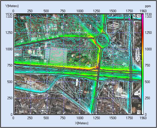
Color contour lines (Wind Angle =45^o)

● Ex-2. Marginal Tietê and Avenida Santos Dumont in São Paulo, Brazil (background map: Google Earth satellite map, see more figures under different wind directions click Albums);

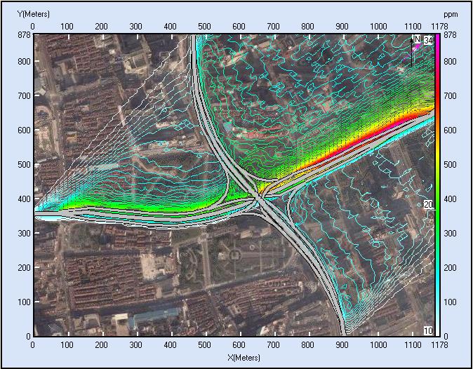
Color contour lines (Wind Angle =135^o)

● Ex-3. Two highways' intersection at the center of Shang Hai (Yan-An Road and Cheng-Du Road), China (background map: Google Earth satellite map, see more figures under different wind directions click Albums);

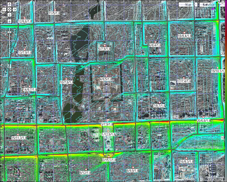
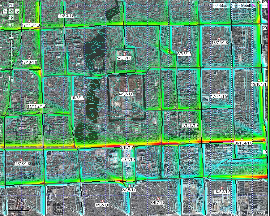
Color contour lines (Wind Angle = 225^o)

● Ex-4. Arterial streets of local Bei Jing city zone, China (background map: Google Earth satellite map, see more figures under different wind directions click Albums);

Color contour lines (Wind Angle =60^o)

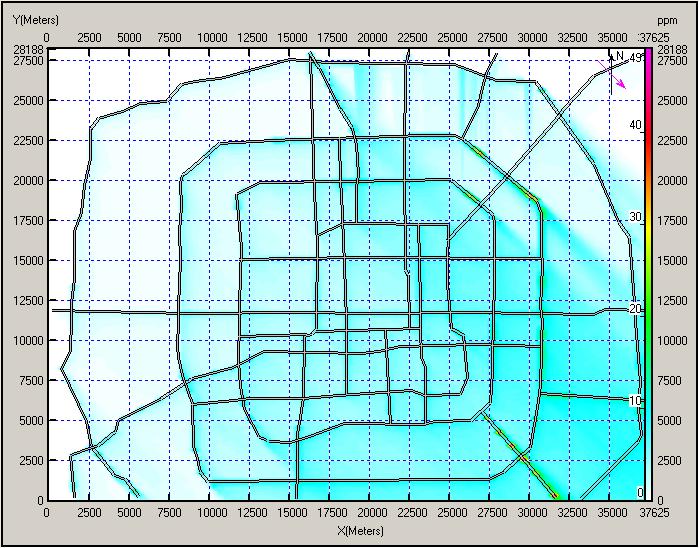
Color contour lines (120^o)

● Ex-5. Highways and arterial streets of Bei Jing city zone, China (background map: Yahoo-China map, see more figures under different wind directions click Albums);

Color contour lines (Wind Angle =315^o) with a rectangle (brown ), specified by the user through the drawing tool provided by software. The position of this region and corresponding characteristic concentrations (maximum, minimum and mean) can be instantly displayed on table.

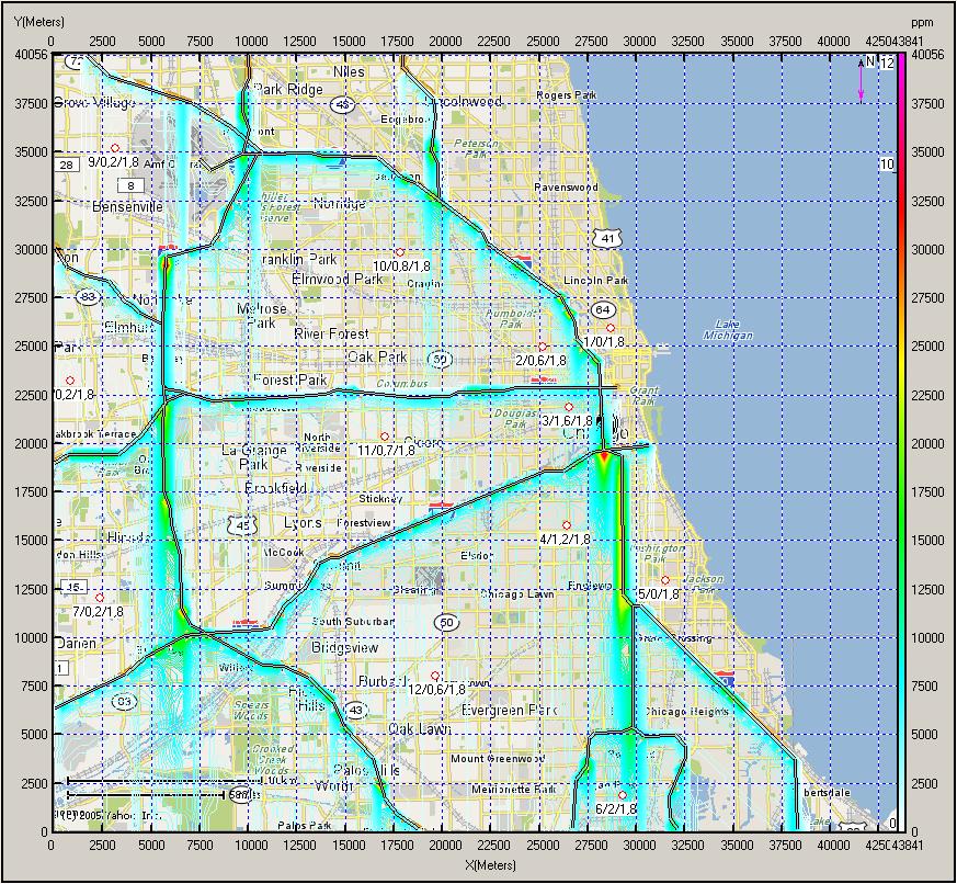
Color filled image (Wind Angle =315^o)

● Ex-6. Highways in Chicago city zone, USA (background map: Yahoo map, see more figures under different wind directions click Albums);

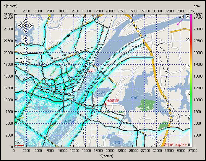
Color contour lines (Wind Angle =0^o)

● Ex-7. Highways and arterial streets of Wu Han city zone, China (background map: Yahoo-China map, see more figures under different wind directions click Albums)

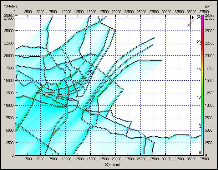
Color contour lines (Wind Angle =45^o)

Color filled image (Wind Angle=45^o)

Top