Once the experimental apparatus has been built, as described in Chapter 4, in the absence of the sample, the CCD should be illuminated in a quite uniform way. As a matter of fact, the illumination is never completely uniform, primarily because of the interference of the main beam with stray light. A typical image is shown in Fig. 6.1. We can easily see some sets of concentric circles, each due to reflections inside a lens, along with speckle patterns properly due to stray light.
When the the sample is placed in the right position, we acquire about
one hundred images for each measurement. The electronic shutter of
the CCD and its interlacement time must be so short that no evident
evolution of the system happens during the exposure: for the samples
we studied, an interlacement delay of
![]() is sufficient. Moreover, different images must be completely
uncorrelated. For a
is sufficient. Moreover, different images must be completely
uncorrelated. For a
![]() colloid, images must be grabbed at
intervals longer that one minute, if only brownian movements are the
source of decorrelation, while for the non equilibrium fluctuations we
studied the images can be taken at intervals of
colloid, images must be grabbed at
intervals longer that one minute, if only brownian movements are the
source of decorrelation, while for the non equilibrium fluctuations we
studied the images can be taken at intervals of
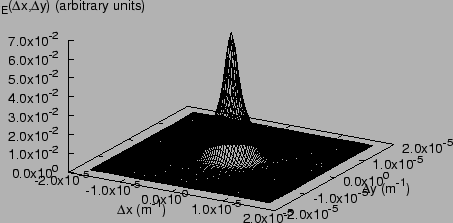
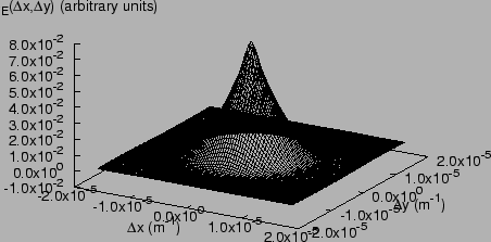
![]() . In
figure 6.2 and
6.3 we show two typical ENFS images,
generated by the interference of the main beam with the light
scattered by colloids of
. In
figure 6.2 and
6.3 we show two typical ENFS images,
generated by the interference of the main beam with the light
scattered by colloids of
![]() and
and
![]() .
The images show a
mean intensity, modulated by the interference with the speckle
pattern. We can notice the different typical size of the
speckles. The set of concentric circles can be seen yet: the stray
light will be removed with the following step.
.
The images show a
mean intensity, modulated by the interference with the speckle
pattern. We can notice the different typical size of the
speckles. The set of concentric circles can be seen yet: the stray
light will be removed with the following step.
Once the images
![]() have been acquired, they are
averaged, in order to evaluate
have been acquired, they are
averaged, in order to evaluate
![]() and
and
![]() . By using
Eq. (6.7), we evaluate
. By using
Eq. (6.7), we evaluate
![]() , the heterodyne signal. Figures
6.4 and
6.5 show the heterodyne signal:
since
, the heterodyne signal. Figures
6.4 and
6.5 show the heterodyne signal:
since
![]() is negative, for some points, a constant
intensity has been added. The images thus simply represent the ENFS
images, cleaned from stray light and optical imprefections.
is negative, for some points, a constant
intensity has been added. The images thus simply represent the ENFS
images, cleaned from stray light and optical imprefections.
The heterodyne signal of each image is then elaborated in order to
obtain its power spectrum. Simple Fourier transforming of the signal
would be uncorrect, due to border effects. First of all, we evaluate
the correlation function. This operation is quite fast, since we can
use a Fast Fourier Transform (FFT) algorithm. An FFT algorithm allows
to evaluate the Fourier tranform of an ![]() matrix, with a
number of arithmetic operations proportional to
matrix, with a
number of arithmetic operations proportional to
![]() . By using Perceval relation, we can obtain the
correlation function by doing an FFT, evaluating the square modulus,
and doing an Inverse FFT (IFFT). This only requires a number of
operation of the order of
. By using Perceval relation, we can obtain the
correlation function by doing an FFT, evaluating the square modulus,
and doing an Inverse FFT (IFFT). This only requires a number of
operation of the order of
![]() . By scanning every
value of
. By scanning every
value of ![]() , and averaging over every
, and averaging over every ![]() pixels, the
number of operations would be of the order of
pixels, the
number of operations would be of the order of
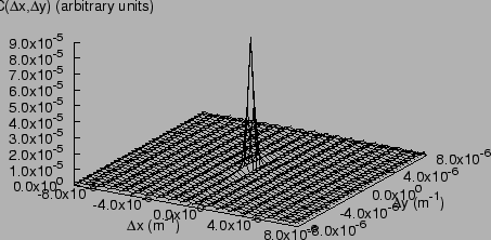
![]() . Using FFT, well known tricks can be used, in
order to correct the boundary effects [19]. Figure
6.6 and
6.7 show the correlation functions thus
evaluated.
. Using FFT, well known tricks can be used, in
order to correct the boundary effects [19]. Figure
6.6 and
6.7 show the correlation functions thus
evaluated.
The correlation function evaluated following the above described algorithm suffers from shot and read noise, that is, for the noise due to the CCD light measurement and acquisition systems. Since such a noise is not correlated to the speckle field due to scattered light, the noise correlation function sums to the speckle correlation function. In order to evaluate the noise correlation function, we acquire a set of about one hundred images, before putting the sample in the system. Then, we apply the above described algorithm to the images, and obtain the correlation function of the noise signal. Figure 6.8 shows the correlation function of the noise signal. We can notice a marked peak in 0, quite narrow, representing the correlation inside a row, and a correlation between lines spaced by two pixels, due to interlacing.
The correlation function of the noise signal is then subtracted by the overall correlation function.
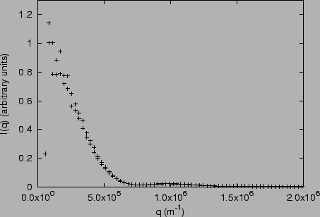
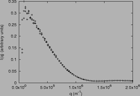
Once the correlation function has been evaluated, through an FFT we
obtain the field power spectrum
![]() . Since our samples
are isotropic, we make an angular average of the power spectra, and
represent our data as a function of the modulus
. Since our samples
are isotropic, we make an angular average of the power spectra, and
represent our data as a function of the modulus ![]() of
of ![]() . The
scattered intensity
. The
scattered intensity
![]() is then obtained by using
Eq. (3.14), that is, simply relating each
value of the power spectra, with wavelength
is then obtained by using
Eq. (3.14), that is, simply relating each
value of the power spectra, with wavelength ![]() to a value of
to a value of
![]() , where the relation
, where the relation
![]() is given by
Eq. (3.13). In
Fig. 6.9 and
6.10 we show the measured
is given by
Eq. (3.13). In
Fig. 6.9 and
6.10 we show the measured
![]() .
.
![\includegraphics[scale=0.4]{ENFS_fondo.ps}](img466.png)
![\includegraphics[scale=0.4]{ENFS_immagine_10um.ps}](img468.png)
![\includegraphics[scale=0.4]{ENFS_immagine_5um.ps}](img469.png)
![\includegraphics[scale=0.4]{ENFS_segnale_10um.ps}](img471.png)
![\includegraphics[scale=0.4]{ENFS_segnale_5um.ps}](img472.png)