Once the experimental apparatus has been built, as described in
Chapter 4, and the sample is placed
in it, we acquire one hundred images. The electronic shutter of
the CCD and its interlacement time must be so short that no evident
evolution of the system happens during the exposure: for the samples
we measured, that is colloids some microns large, with brownian
movements, and non equilibrium fluctuations in the free diffusion of
simple liquids, an interlacement delay of
![]() is sufficient. Moreover, different images must be completely
uncorrelated. For a
is sufficient. Moreover, different images must be completely
uncorrelated. For a
![]() colloid, images must be grabbed at
intervals longer than one minute, if only brownian movements are the
source of decorrelation. For the non equilibrium fluctuations we
studied, the interval was about one second.
colloid, images must be grabbed at
intervals longer than one minute, if only brownian movements are the
source of decorrelation. For the non equilibrium fluctuations we
studied, the interval was about one second.
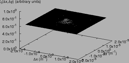
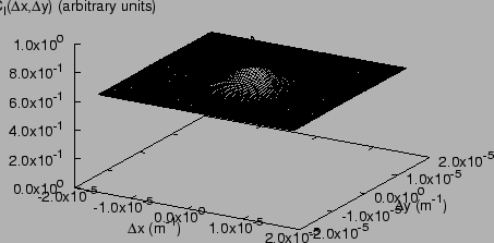
In figure 5.1 and
5.2 we show two typical images of the
near field intensity of the light scattered by colloids of
![]() and
and
![]() .
We can notice the different typical size of the speckles.
.
We can notice the different typical size of the speckles.
For each image, we evaluate the correlation function. This operation
is quite fast, since we can use a Fast Fourier Transform (FFT)
algorithm. An FFT algorithm allows to evaluate the Fourier tranform of
an ![]() matrix, with a number of arithmetic operations
proportional to
matrix, with a number of arithmetic operations
proportional to
![]() . By using Perceval relation,
we can obtain the correlation function by making an FFT, evaluating the
square modulus, and making an Inverse FFT (IFFT). This only requires a
number of operation of the order of
. By using Perceval relation,
we can obtain the correlation function by making an FFT, evaluating the
square modulus, and making an Inverse FFT (IFFT). This only requires a
number of operation of the order of
![]() . By
scanning every value of
. By
scanning every value of ![]() , and averaging over every
, and averaging over every ![]() pixels, the number of operations would be of the order of
pixels, the number of operations would be of the order of
![]() . Using FFT, care must be taken in order to
correcly evaluate the correlations near the boundarys: FFT assumes
periodic boundarys, so the image must be embedded in a bigger
matrix, filled with zeroes. Since the FFT is faster if
. Using FFT, care must be taken in order to
correcly evaluate the correlations near the boundarys: FFT assumes
periodic boundarys, so the image must be embedded in a bigger
matrix, filled with zeroes. Since the FFT is faster if ![]() and
and
![]() are powers of 2 [19], we used a matrix of
are powers of 2 [19], we used a matrix of
![]() points. After the correlation function has been evaluated, we normalize
it, by dividing by the number of independent couples used to evaluate
the correlation function.
points. After the correlation function has been evaluated, we normalize
it, by dividing by the number of independent couples used to evaluate
the correlation function.
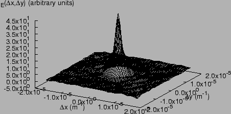
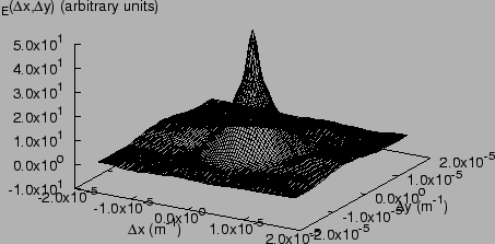
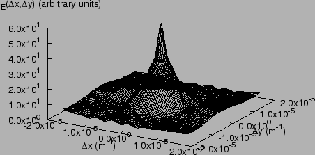
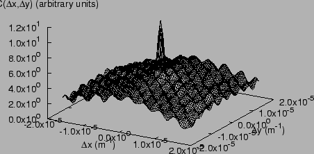
The correlation functions of every image are averaged, thus obtaining
![]() . Fig. 5.3 and
5.4 show typical graphs of the intensity
correlation function
. Fig. 5.3 and
5.4 show typical graphs of the intensity
correlation function
![]() , for a colloid
made of polystyrene spheres with diameters of
, for a colloid
made of polystyrene spheres with diameters of
![]() and
and
![]() . We can notice that the correlation function has a maximum
at
. We can notice that the correlation function has a maximum
at
![]() , then decreases, until it reaches the plateau
value, about one half the peak value. This behaviour is typical of
every speckle field.
, then decreases, until it reaches the plateau
value, about one half the peak value. This behaviour is typical of
every speckle field.
Neglecting the stray ligth, we could evaluate the field correlation function by using the Siegert relation, Eq. (3.65):
 |
(5.16) |
|
|
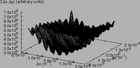
In order to subtract the contribution of the stray light, we evaluate
the correlation function of the average of all the images, thus
obtaining
![]() . The evaluation of
the correlation function is obtained with the above described
algorithm. In Fig. 5.7 and
5.8 are shown typical graphs of the
correlation function of the mean intensity, for the two colloids. The
graphs are not flat, due to the stray light.
. The evaluation of
the correlation function is obtained with the above described
algorithm. In Fig. 5.7 and
5.8 are shown typical graphs of the
correlation function of the mean intensity, for the two colloids. The
graphs are not flat, due to the stray light.
|
|
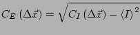
Through Eq. (5.23) we evaluate
![]() , under the hypothesis that both the
stray light field and the scattered light field have a real and
positive correlation function. Typical field correlation function,
corrected for the stray light using
Eq. (5.23), are shown in figure
5.9 and 5.10: we
can notice a signitificative increase in the smoothness of the graphs,
with respect to Fig. 5.5 and
5.6.
, under the hypothesis that both the
stray light field and the scattered light field have a real and
positive correlation function. Typical field correlation function,
corrected for the stray light using
Eq. (5.23), are shown in figure
5.9 and 5.10: we
can notice a signitificative increase in the smoothness of the graphs,
with respect to Fig. 5.5 and
5.6.
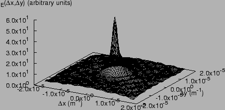
We apply a Fourier tranform to the two dimensional correlation
function
![]() , thus obtaining the field
power spectrum
, thus obtaining the field
power spectrum
![]() . Since our samples are isotropic,
we make an angular average of the power spectra, and represent our
data as a
function of the modulus
. Since our samples are isotropic,
we make an angular average of the power spectra, and represent our
data as a
function of the modulus ![]() of
of ![]() . The scattered intensity
. The scattered intensity
![]() is then obtained by using
Eq. (3.14), that is, simply relating each
value of the power spectra, with wavelength
is then obtained by using
Eq. (3.14), that is, simply relating each
value of the power spectra, with wavelength ![]() to a value of
to a value of
![]() , where the relation
, where the relation
![]() is given by
Eq. (3.13). In
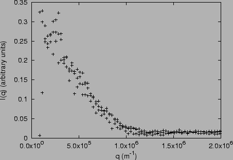
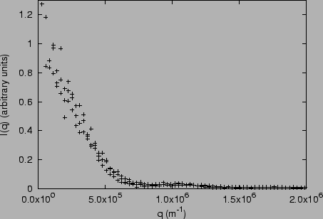
Fig. 5.11 and
5.12 we show the measured
is given by
Eq. (3.13). In
Fig. 5.11 and
5.12 we show the measured
![]() .
.
![\includegraphics[scale=0.4]{result_2d_imm_5um.ps}](img410.png)
![\includegraphics[scale=0.4]{result_2d_imm_10um.ps}](img411.png)