Correction for finite samples.

In order to evaluate the correlation function of the mean intensity, we average a given amount of images, then we evaluate the correlation function of the obtained mean value. Since the number of images we average is finite, the correlation function will not correspond to that of eq. (5.14). For example, if the stray light vanishes, the mean intensity will still present fluctuations, due to the scattered light. These fluctuations vanish as the square root of the number of the averaged images, and consequently the correlation function becomes flat only for infinite samples.

A similar problem arises when working with a stochastic, gaussian variable. If we have $N$ values of the stocastic variable $x$, distributed with probability $P\left(x\right)\propto \exp\left[-\left(x-x_0\right)/ \left(2\sigma^2\right)\right]$, we find that the best value for $x_0$ is the mean of the values $x$, and the best value for $\sigma$ is the root mean square displacement of the values $x$ from $x_0$. On the other hand, the average on a finite number of elements will be displaced from $x_0$ of an amount, vanishing as the square root of the number of the samples $N$, but so that the root mean square displacement of the data from the mean is alwais smaller than $\sigma$. It is thus necessary to use the Bessel correction, dependent on the number of the samples $N$.

Generally the Bessel correction is obtained in consequence of the ``maximum likelihood'' condition. This means that, given a set of values of a stochastic variable, and given a family of probability distributions, the parameters of the family must be selected in order to maximize the probability of finding the given data. Another approach is to find a suitable algorithm which gives the values of the parameters, from a set of data. The algorithm will be selected in order that the output values will be distributed around the true ones, with minimum square displacement. For a gaussian distribution, the two approaches give the same result. It is easy to show that, for example for a Heaviside distribution, the maximum likelihood condition fails to obtain the best results.

In our case, the distribution function of the intensity is not gaussian. We will use weak condition, that is, we will look for an algorithm giving values which average to the true ones. In other words: we will try to avoid sistematic erroneous evaluations of the correlation function.

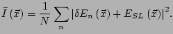
We define $\bar{\cdot}$ as the mean over $N$ samples. In particular $C_{\bar{i}}$ is the correlation function of the averaged $N$ images. To avoid sistematic errors, we must first evaluate $\left\{C_{\bar{I}}\right\}$:

$$\left\{C_{\bar{I}}\left(\Delta \vec{x}\right)\right\} = \left\{ \... ...t(\vec{x}\right) \bar{I}\left(\vec{x} + \Delta \vec{x}\right) \right> \right\},$$ (5.11)

where the average intensity of $N$ images $\bar{I}$ is given by the sum of the field scattered by the sample $\delta E\left(\vec{x}\right)$ and the field of the stray light $E_{SL}\left(\vec{x}\right)$:

$$\bar{I}\left(\vec{x}\right) = \frac{1}{N} \sum_n {\left\vert \delta E_n\left(\vec{x}\right) + E_{SL}\left(\vec{x}\right) \right\vert^2}.$$ (5.12)

So we obtain:

$$\left\{C_{\bar{I}} \left(\Delta \vec{x}\right)\right\} = \frac{1}... ...c{x}\right)E_{SL}\left(\vec{x}+\Delta\vec{x}\right) \right] \right> \right\} }.$$ (5.13)

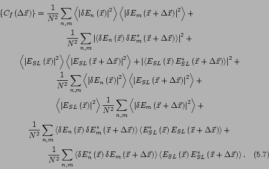
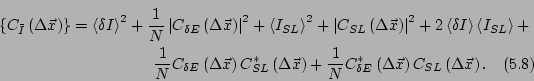
We can follow the calculations performed in Section 5.1 to obtain Eq. ( 5.8). In this case we obtain:

$$\begin{multline} \left\{C_{\bar{I}}\left(\Delta \vec{x}\right)\right\} = \frac{1... ...\vec{x}\right)E_{SL}^*\left(\vec{x}+\Delta\vec{x}\right) \right>. \end{multline}$$

The mean values can be calculated, provided that the two cases, $n=m$ and $n\ne m$ are taken into account:

$$\begin{multline} \left\{C_{\bar{I}}\left(\Delta \vec{x}\right)\right\} = \left<\... ... E}^*\left(\Delta\vec{x}\right) C_{SL}\left(\Delta\vec{x}\right). \end{multline}$$

The result reduces to eq. (5.14) in the limit $N\to \infty$:

$$\left\{C_{\bar{I}}\left(\Delta \vec{x}\right)\right\} = \left( \l... ...}\left(\Delta \vec{x}\right) + C_{SL}\left(\Delta \vec{x}\right)\right\vert^2 .$$ (5.14)

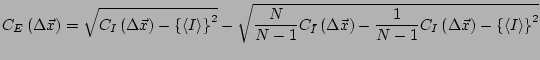
From eq. (5.8), (5.22) and (5.15) we can evaluate the field correlation function:

$$C_E\left(\Delta \vec{x}\right) = \sqrt{C_I\left(\Delta \vec{x}\ri... ...rac{1}{N-1}C_I\left(\Delta \vec{x}\right) - \left\{ \left< I\right>\right\}^2 }$$ (5.15)

Hosted by www.Geocities.ws