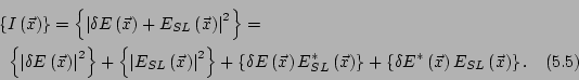
From a set of ONFS images
![]() ,
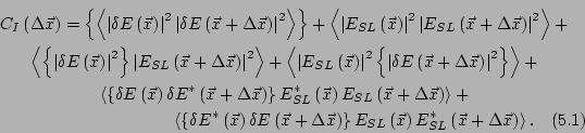
we can measure the intensity correlation function:
,
we can measure the intensity correlation function:
| (5.1) |
| (5.2) |
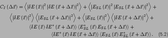
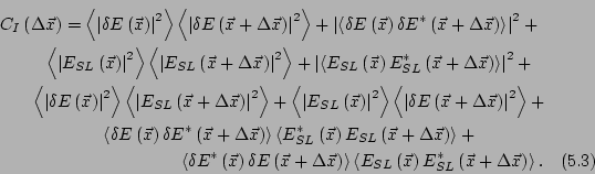
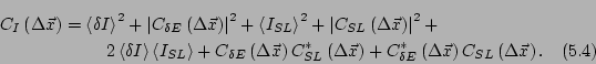
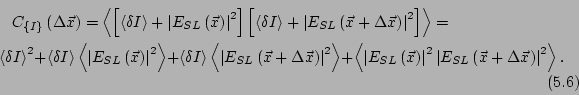
![$\displaystyle C_I\left(\Delta \vec{x}\right) = \left\{ \left< \left[ \left\vert...
...ec{x}\right) E_{SL}\left(\vec{x}+\Delta\vec{x}\right) \right] \right> \right\}.$](img370.png) |
(5.3) |
Since
![]() is a random, circular gaussian field,
the mean over different images of its odd powers
vanishes; since
is a random, circular gaussian field,
the mean over different images of its odd powers
vanishes; since
![]() is static, it can be
considered as a costant,
with respect to
is static, it can be
considered as a costant,
with respect to ![]() , the average on the images:
, the average on the images:
Since both
![]() and
and
![]() are gaussian fields, we can use Siegert relation
Eq. (3.65) to express four-point correlation
functions in terms of two-point ones.
are gaussian fields, we can use Siegert relation
Eq. (3.65) to express four-point correlation
functions in terms of two-point ones.
We define
![]() ,
,
![]() ,
,
![]() ,
,
![]() :
:
The result is that the stray light field correlation sums to the scattered field correlation:
In order to obtain informations about the correlation of the stray light field,
we acquire a great number of images, with different scattered field, and
we average them, thus obtaining the correlation function of the mean intensity
![]() . Then, we measure the correlation
function of the mean intensity:
. Then, we measure the correlation
function of the mean intensity:
| (5.5) |
We evaluate the mean intensity
![]() :
:
Since ![]() does not depend on the image:
does not depend on the image:
| (5.6) |
Using the gaussian properties of the scattered light:
Now we can evluate the correlation function of the mean intensity:
From eq. (5.12), we can evaluate the mean value of the intensity of the images:
Eq. (5.8), (5.14), (5.15) give some informations about the field correlation of the scattered and stray light. If both the correlation functions are real and positive, the best evaluation of the field correlation function of the scattered field is:
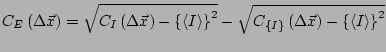 |
(5.10) |