Rebound Of Hollow Elastic Spheres

Last updated: July 20, 2002
Rebound Of Hollow Elastic Spheres

The vibrational mode frequencies and coefficient of restitution are studied for a hollow elastic sphere from molecular dynamics simulations of spherical clusters of up to 13,500 atoms. The results are applied to calculate the ideal characteristics of a ping pong ball. Both a solid sphere and a thin shell have minimal conversion of energy to vibrational modes during a bounce, but energy loss is maximized when the inner radius is approximately 0.75 times the outer radius.

   Hollow spheres are of interest because some kinds of balls (e.g. tennis [Cross 2002 pdf ::], ping pong [Hubbard and Stronge 2001 ::] ) are hollow spheres rather than solid spheres, and sometimes the question is casually raised as to whether being hollow affects the way a ball bounces [Brooks 2001 link to article] [PBS TV link].
   Spheres whose material properties are functions of the radial coordinate (ρ(r), Y(r), ...) are studied in geophysics and seismology [Hanyk et al. 1998 pdf ::]. The special case of a uniform elastic sphere has been extensively studied [Ye 2000 pdf ::] and solved exactly [Murray 2002 link to article].
   The present article addresses only the situation of a hollow sphere with uniform material properties. We are unaware of previous studies of this specific problem, except the limits of a solid sphere [Murray 2002 link to article] and the limit of a thin shell [Niordson 1987]. The notation used is as follows: The outer radius of the sphere is R. The inner radius is r_in. I define b = r_in/R. The sphere is made from isotropic elastic material with Young's modulus Y, density ρ and Poisson ratio ν. The sphere is dropped (down the y-axis) moving with speed v just before it hits the floor, which is assumed to be infinitely hard. Vibrational modes of the sphere have frequency f.
   The number of atoms in the sphere is N. The atoms are assumed to interact through a model potential U(r). Two different models of inter-atomic forces are used, the Lennard Jones potential and the Quadratic potential [Murray, 2002 link to article]. The time step in the computer simulations is dt_sim. Where animations are shown, the simulation time per animation frame is dt_ani. The animations should appear on your browser at 10 frames per second. There is no gravitation in the simulations. The upward force from the floor during the bounce is F(t). The compression distance is y (i.e. y = R - height of cm above floor). The duration of the collision is T.
   The properties of of the simulated material are as shown in the table below:

Linear Elastic Properties of Molecular Dynamics Solid:
Property	Symbol	Average value	Unit	Min. value	Max. value	Relation:
Mass of one atom	m_atom	1.0000000	kg	(exact)
Density	ρ	1.0000000	kg/m³	(exact)
Atomic force constant	dF/dr	1.0000000	N/m	(exact)
Atom center-center distance	d_cc	1.1224621	m	(exact)		d_cc=(sqrt(2)m_atom/ρ)^1/3
Bulk Modulus	B	0.8399473	Pa	(exact)		2ρ(d_cc)²(dF/dr)/(3m_atom)
Young's Modulus	Y	1.215	Pa	1.172	1.261	(use md4ym.cpp)
Poisson's ratio	ν	0.2589	- - -	0.250	0.267	ν=(3B-Y)/(6B)
Shear Modulus	G	0.4826	Pa	0.4623	0.5045	G=3BY/(9B-Y)
1st Lamé constant	λ	0.5182	Pa	0.5036	0.5317	λ = B - (2/3)G
Shear wave speed	C_s	0.6947	m/s	0.6799	0.7103	C_s=sqrt(G/ρ)
Longitudinal wave speed	C_l	1.2179	m/s	1.2068	1.2299	C_l=sqrt((λ+2G)/ρ)
C_s/C_l		0.5704	- - -	0.5634	0.5775

At right is an animation of a hollow sphere dropped with speed 0.030 m/s. R = 10 and N = 3672 atoms. b = r_in/R = 0.5. The rebound speed is 0.0292 m/s. dt_sim=0.2 s and dt_ani=5s. The frames are displayed 10 per second. The Lennard Jones potential was used. The maximum strain was 0.366. Almost none of the initial center of mass kinetic energy is lost. Only a central cross section of the sphere is shown here. (md2graf7.cpp fig2c.gif)

At left is a hollow sphere dropped with initial speed 0.030 m/s. R = 19.4, N = 10430, and b = 0.87. The rebound speed is 0.0296 m/s. dt_sim=0.2 s. dt_ani=5s. The Lennard Jones potential was used. The maximum strain was 0.438. Only a central cross section of the sphere is shown here. This is similar to a ping pong ball, which is a thin but rigid shell. The gentle, long duration the collision does not allow vibrational modes to be excited. (md2graf7.cpp fig2d.gif)

At right is a hollow sphere dropped at 0.030 m/s. R = 15.5, b = 0.7 and N = 10188. The rebound speed is 0.0282 m/s. dt_sim=0.2 s. dt_ani=5s. The frames are displayed 10 per second. The Lennard Jones potential was used. The maximum strain was 0.532. In this case, some excitation of the vibrational modes can be seen, which corresponds to the energy loss. The mode excited is the vertical axial stretch mode. (md2graf7.cpp fig2e.gif)

Shown above are results of dropping hollow spheres with varying ratios of inner to outer radius. In each case N = 13300. The initial speeds are as shown. The quadratic potential was used. The purple dots show the ratio of final to initial mechanical energy on a scale from 0 to 1. The yellow dots show contact time over radius on a scale from 0 to 20. The blue dots show the maximum strain. The sudden drop in energy ratio when b > 0.9 is likely as a result of the thickness of the shell dropping below 2. (md4.cpp hs2.dat hs3.dat hs4.dat plot4.cpp hs2.gif hs3.gif hs4.gif)

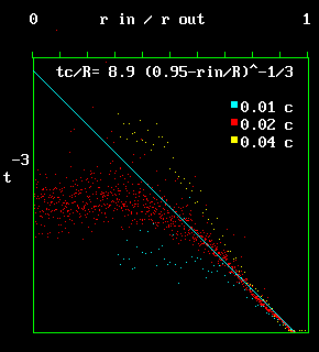
The inverse cube of the collision time is plotted for three different speeds (see colour code legend) as a function of b. Although collision time is speed dependent for a solid sphere, it appears to become independent of speed for a thin spherical shell. (hs2.dat hs3.dat hs4.dat plot5.cpp hs10.gif)

T =

8.9 R (0.95 - b)^-1/3

(Thin shell)

[..c..]

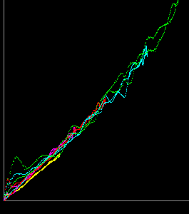
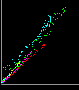
At right acceleration is plotted versus compression distance for a hollow sphere with b = 0.9, N = 13452 and R = 22.9. The initial speeds are: yellow=0.005 m/s,purple=0.0071 m/s, red=0.01 m/s, blue=0.014 m/s, green=0.02 m/s. The quadratic potential is used. Both "loading" and "unloading" are shown. Generally, force seems to be linearly proportional to compression. This is much different from the situation for a solid sphere where Hertz predicted F proportional to y^1.5. The jagged shape is likely due to the thickness of the shell being only 2.07. Depending on the orientation, this would be just 2 to 3 atomic layers thick. (md4avsy.cpp hs5.gif)

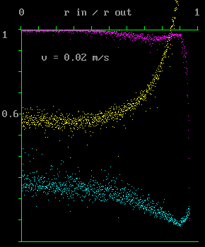
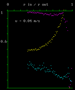
In this figure (left) N = 9972, R=20.7, b=0.9 and the quadratic potential was used. dt_sim=0.5. The colour code for speed is the same as in the previous figure. the small radius results in less smoothness in the curves. (md4avsy.cpp hs7.gif)

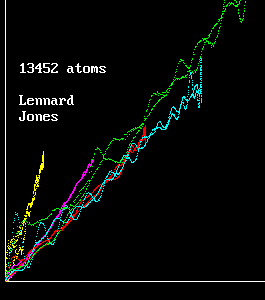
In this figure (right) N = 13452, R=22.9, b=0.9 and this time the Lennard Jones potential was used. dt_sim=0.5. The colour code for speed is the same as in the previous figure. (md4avsy.cpp hs8.gif)

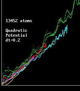
In this figure (left) N = 13452, R=22.9, b=0.9 and the quadratic potential was used. This time dt_sim=0.2 as a check on convergence. High frequency oscillations are believed to be an artifact. They are also present when dt_sim=0.5 but are removed by two point boxcar averaging. The colour code for speed is the same as in the previous figure. (md4avsy.cpp hs9.gif)

Vibrational Mode Frequencies

This shows the frequency of the lowest axial stretch vibrational mode versus the inner to outer radius ratio. The data is fit by the blue line whose formula is equation [..a..]. All spheres had approximately 13,500 atoms. The mode was excited by stretching the sphere along one axis. For the last data point (b=0.94), R was 26.7 making the thickness of the shell just 1.60. The spectrum changes completely if b is made any larger, suggesting that the sphere loses its structural integrity. The quadratic potential was used. dt_sim=0.5. 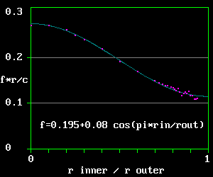(md4mod.cpp fvsrr.cpp hs6.gif)

f lowest = (1/R)(0.195 + 0.08 cos(π b))

[..a..]

Taken together, the above two figures suggest that the situation for a thin shell is well approximated as a linear force as a function of compression. Also, the vibrational frequency in the thin shell limit approaches

f lowest = 0.115/R

(Thin shell)

[..b..]

   Initially I found it very surprising that the vibrational frequency does not approach zero in the limit that the shell becomes very thin.

Ping Pong Balls

   For a ping pong ball with official size R=20 mm (www.school-for-champions.com) and made out of celluloid (also called cellulose nitrate) which has a Young's modulus (Elastic Modulus) Y = 1311 to 1518 MPa� (www.efunda.com) and density 1350 to 1400 kg/m³. I was unable to find any information about the Poisson ratio of celluloid. Vibrational frequencies are more closely related to the shear modulus than to Young's modulus. However, celluloid is a hard plastic, and is not a kind of rubber. Therefore the Poisson ratio of celluloid can be expected to be in the vicinity of 0.3. If I make the rough approximation that its Poisson ratio is exactly 0.2589, then celluloid is "similar" to the molecular dynamics solid. In that case, things simply scale according to the density and Young's modulus. For a material with Young's modulus Y and density ρ, the frequency from molecular dynamics is multiplied by sqrt(Y/(1.215 ρ)) where 1.215 is the Young's modulus of the molecular dynamics solid.
So based on equation [..b..] its lowest vibrational frequency should be f = sqrt(1.41e9/((1.215)(1370))) 0.115 / 0.02 = 5290 Hz.
   Based on its official diameter of 40 mm, the outer surface area of a ping pong ball is 0.0050 m². Based on its mass of 2.7 g, (www.school-for-champions.com) and the density of celluloid, its volume is 1.96E-6 m³. Thus the thickness of a ping pong ball is 0.40 mm, and so b for a ping pong ball is 0.980.
   Equation [..c..] is not directly suitable when b is 0.98, since it becomes singular at 0.95, which is the point at which the shell becomes too thin. If the sphere had many more atoms, then this point would come at a ratio closer to one. So my guess for the asymptotic formula in the limit of many atoms is:

T =

8.9 R (1 - b)^-1/3

(Thin shell)

[..d..]

   Applying this to the ping pong ball, the duration of its bounce with a hard table should be 0.00071 s. (0.71 ms). This appears to be something that could be determined for an actual ping pong ball. At this time duration, the dominant Fourier components of F(t) should have frequencies up to about 1400 Hz. The gap between this frequency and the lowest vibrational frequency of the ping pong ball (5290 Hz, calculated above) means that excitation of vibrational modes is not an important mechanism for energy loss of a ping pong ball. (However, it would be nice to analyze the Fourier components of the force and see how small the amplitude actually is at that frequency)
   For a ping pong ball dropped 30 cm, the formula v² = 2 g h (where g=9.8 m/s²) gives its speed at impact as 2.42 m/s. Its maximum acceleration (at the point of maximum compression) assuming the force is linearly proportional to the compression distance, will be 10700 m/s². The maximum distance by which the ball is compressed will be 0.00055 m (0.55 mm). The maximum upward force on the ball from the table is 28.9 Newtons (6.5 pounds of force). All of these calculations assume that the ping pong table is infinitely hard.
   Apparently, part of the rules for ping pong include a lower limit on the coefficient of restitution, based on the requirement that "a standard ping-pong ball falling down from a height of 30 cm should bounce back at least 23 cm." (link here) This corresponds to a coefficient of restitution of 0.876. It would be interesting to check what the range of coefficient of restitution is for actual ping pong balls.

Higher Frequency Vibrational Modes:

   Doing a more careful search for vibrational modes when b=0.75, I found the following: (using md4mod.cpp) f = 0.141/R, 0.146/R, 0.155/R, 0.200/R, 0.217/R, 0.225/R, 0.241/R, etc. The last three are toroidal modes (Love waves). I suspect that the lowest two are axial stretch modes, but haven't confirmed that. So toroidal modes are not the lowest frequency modes for a thin shell.
   The lowest modes of a shell of b = 0.90 (using md4mod.cpp) are f = 0.118/R, 0.138/R, 0.145/R, 0.157/R, 0.162/R, 0.175/R, 0.184/R, etc. Given the thinness of the shell these values are not precise, and they vary from sphere to sphere.
The axial mode is not the lowest mode for small b, but it is the lowest mode for large b.

Excitation of Vibrational Modes During a Bounce:

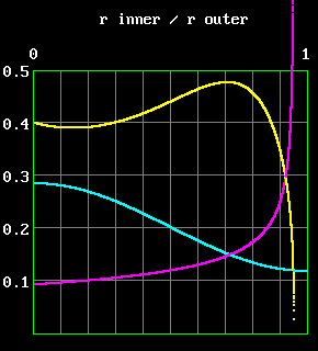
The blue curve at left is a plot of equation [..a..] for the lowest axial stretch mode vibrational frequency. The horizontal axis is the ratio of inner to outer radius. The purple curve is a plot of equation [..c..] for the collision time. The yellow curve is the blue curve divided by the purple curve. The peak is reached at about 0.70. It is at this ratio that maximum energy loss should occur. The vertical axis scale refers only to the yellow curve. (plot6.cpp hs11.gif)

The actual motion of a ping pong ball in play includes rotation. Also, the ball does not hit at normal incidence. The idealization of the table as being infinitely hard needs to be examined. The friction between the ball and the table as well as the dissipative characteristics of the plastic would need to be included in a realistic model of a ping pong ball bounce.

References:

Rod Cross, "Measurements of the horizontal coefficient of restitution for a superball and a tennis ball" Am. J. Phys. 70, 2002 p.482-489 pdf ::

Patrick Brooks, "Which ball bounces higher, a solid or a hollow ball?" Country School 15 June 2001 link to this (A description of an 8th grade science project comparing solid and hollow ball bounces. His initial guess was that hollow balls should bounce less high, but he found the opposite among the balls he tested.)

Corrine Lowen et al. "On the ball" Public Broadcasting Service link. (They simply suggest that "hollow" and "solid" balls should be used without suggesting what difference it should make.)

Niordson, Frithiof I., "The Spectrum of Free Vibrations of a Thin Elastic Spherical Shell" (November 1987). Int. J. Solids Structures, Vol. 24, No. 9, pp. 947-961, 1988.

L. Hanyk, C. Matyska and D. A. Yuen "Initial value approach for viscoelastic responses of the earth's mantle" 1998. pdf ::

Zhen Ye, "On the Low Frequency Elastic Response of a Spherical Particle" Chinese Journal of Physics Vol. 38, pages 103-110, (2000). link to pdf ::

Daniel B. Murray, "Coefficient of Restitution Of a Spinless Elastic Sphere Bouncing at Normal Incidence on a Hard Surface" 2002 link to article

Daniel B. Murray " Vibrational Frequencies of an Elastic Sphere" 2002 link to article

M. Hubbard and W. J. Stronge, "Bounce of Hollow Balls on Flat Surfaces" Sports Engineering 4, 49-61 (2001) ::

------------------------
link here
"...pong-pong balls...are made of nitrocellulose and a small percentage of camphor..."

link here
HISTORY OF U.S. TABLE TENNIS
"turn-of-the-century innovation of the celluloid ball, "

PING-PONG BALLS link here
In 1880, the celluloid ball was invented by English engineer James Gibb. A modern official table-tennis ball used to have a diameter of 38 mm, but nowadays 40mm, and weighs 2.5 gr. It has to be made of celluloid or a similar synthetic material, and has to be white, yellow or orange. ...a standard ping-pong ball falling down from a height of 30 cm should bounce back at least 23 cm.
-----------------------------
Ping pong balls link here
The ball should have a diameter of 40 mm., weigh 2.7 gm. and be made of celluloid or similar plastic material. It can be white or orange.
--------------------------------
link here
Celluloid - From Billiard Ball to Ping Pong Ball...
"Celluloid is a semi-synthetic material; a mixture of camphor and nitrocellulose " "Having progressed from it�s beginnings as a billiard ball, there is some irony in the fact that Celluloid�s biggest application today is in Ping Pong balls, and not much else."
------------------------
Properties of Cellulose Nitrate (Celluloid) link here
Elastic Modulus (MPa)� 1311 - 1518
Tensile Strength (MPa)� 48 - 55
Compressive Strength (MPa) at yield or break� 14 - 55
Elongation at break (%)� 40 - 45
Specific Gravity�1.35 - 1.4
---------------------
Toys: cannot be made of cellulose nitrate. link here
-----------------------
Properties of Cellulose Nitrate (Celluloid) link here
Tensile strength 35 (min) 70 (max) MPa
Elongation 10 (min) 40 (max) %
Density 1350 (min) 1400 (max) kg/m3
--------------
From www.matweb.com
Cellulose Nitrate, Molded
Density 1.4 g/cc
Tensile Strength, Yield 50 MPa
Elongation @ break 40 %
Tensile Modulus 15 GPa [seems too high by10x !?]
------------------
Cellulose nitrate = nitrocellulose = gun cotton
-------------------
http://www.soldana.com/eng/ordliste__hvad_er_det_.htm
Cellulose-nitrate is used for manufacturing table tennis balls and cellulose-acetate films for photography.
------------
http://www.exploratorium.edu/baseball/bouncing_balls.html
Has chart showing rebound of table tennis ball is 15% (so that coef. of restitution is only 0.38) !!!
---------------------------------
http://www.oxfordcroquet.com/tech/testing/index.asp
Croquet balls:
Coefficient of restitution (bounce) 35-45" rebound when dropped from 60" (Laws of Croquet Appendix 2). Mallet - Ball contact times single ball strokes=~1ms Croquet stroke= ~2.9ms Ball - Ball contact times approximately 1.8ms
------------------------
http://www.physast.uga.edu/~mgeller/dartmouth-nano.pdf
Michael R. Geller et al. "Theory of electron-phonon dynamics in insulating nanoparticles" 11 July 2001
"An isolated spherical nanoparticle of diameter d cannot support internal vibrations at frequencies less than the so-called Lamb mode frequency, about 2 π vt / d where vt is the bulk transverse sound velocity." (Reference: H. Lamb, Proc. London Math. Soc. 13, 187 (1882).)
-------------------------
http://www.ndt-ed.org/EducationResources/CommunityCollege/Ultrasonics/Physics/elasticsolids.htm
Shear (transverse) wave velocity can be written as sqrt(c44/ρ). For steel 0.32 cm/microsecond. Shear velocity is approximately one half that of compressional
(guess: c44 = shear stress/shear strain?) --------------------------
http://www.geoforum.com/knowledge/texts/compaction/viewpage.asp?ID=13
G = CS CS ρ
CS = shear wave velocity, ρ = bulk density, G = shear modulus
----------------------------------
M. Rauterberg et al. "Automatic sound generation for spherical objects hitting straight beams based on physical models"
www.ipo.tue.nl/homepages/mrauterb/ publications/EDMEDIA94paper.pdf
in which they mention
---------------

Daniel Murray
Associate Professor
Math, Stats & Physics Unit
University of British Columbia - Okanagan
Kelowna, BC, Canada
daniel "dot" murray "at" ubc "dot" ca

Hosted by www.Geocities.ws