Main: The Wave equation

A few problems:

Example:

Consider the one dimensional version of the the example in §8.2. That is, find the solution of the one dimensional wave equation subject to a time harmonic oscillator at the origin which switchs on at t=0.

The problem is to solve

$\begin{displaymath} {1\over c^{2}}{{\partial^2 \phi}\over{\partial {t}^2}} - {{... ...^2 \phi}\over{\partial {x}^2}} = H(t)\delta(x)e^{i\omega t}. \end{displaymath}$

In terms of the Green's function $G(x,t; y,\tau)$ the solution is

$\begin{displaymath} \phi(x,t) = \int^{\infty}_{-\infty}\kern 4pt \int^{\infty}... ... y,\tau) H(\tau)\delta(y) e^{i\omega\tau}\,dy\kern 4pt d\tau. \end{displaymath}$

Since $H(\tau)=0$ for $\tau<0$ and

$\begin{displaymath} \int^{\infty}_{-\infty} G(x,t; y,\tau)\delta(y)\,dy = G(x,t;0,\tau) \end{displaymath}$

we see that

$\begin{displaymath} \phi(x,t) = \int^{\infty}_{0} G(x,t; 0,\tau) e^{i\omega\tau} d\tau. \end{displaymath}$

From (8.8) or (8.9)

$\begin{displaymath} G(x,t; 0,\tau) = {c\over 2}H(t-\tau-\left\vert x\right\vert/c), \end{displaymath}$

hence

$\begin{displaymath} \phi(x,t) = {c\over 2}\int^{\infty}_{0} H(t-\tau-\left\vert x\right\vert/c) e^{i\omega\tau}d\tau. \end{displaymath}$

Now, put

$\begin{displaymath} q=t-\tau-\left\vert x\right\vert/c,\quad dq = -d\tau \end{displaymath}$

$\begin{displaymath} \phi(x,t) = {c\over 2}\int_{-\infty}^{t-\left\vert x\right\... ... H(q)\exp\left(i\omega(t-\left\vert x\right\vert/c-q)\right)dq \end{displaymath}$

If $t-\left\vert x\right\vert/c < 0$ then the integral is zero, since q is always less than zero and hence H(q)=0 over the whole range of integration. All this means is that if $\left\vert x\right\vert > ct$ then the disturbance which switches on at time t=0 and travels at speed c has not had time to reach the point x which is a distance $\left\vert x\right\vert$ from the origin. Thus there is zero disturbance at x.

If $t-\left\vert x\right\vert/c > 0$ then

$\begin{displaymath} \int_{-\infty}^{t-\left\vert x\right\vert/c} H(q)\exp\left... ...{0} \exp\left(i\omega(t-\left\vert x\right\vert/c-q)\right)dq \end{displaymath}$

since H(q)=0 for q<0 and H(q)=1 for q>0. Note that

$\begin{displaymath} \int^{t-\left\vert x\right\vert/c}_{0} \exp\left(i\omega(t... ...right)\int^{t-\left\vert x\right\vert/c}_{0} e^{-i\omega q}dq \end{displaymath}$

and hence

$\begin{displaymath} \int^{t-\left\vert x\right\vert/c}_{0} \exp\left(i\omega(t... ...mega}\left( 1- e^{i\omega(t-\left\vert x\right\vert/c}\right). \end{displaymath}$

This means that if $\left\vert x\right\vert<ct$ then the disturbance has had time to propagate at speed c from the origin to x and it gives the effect of the disturbance.

In total we find that

$\begin{displaymath} \phi(x,t) = {ic\over 2\omega}H(t-\left\vert x\right\vert/c) \left( 1-e^{i\omega(t-\left\vert x\right\vert/c)}\right). \end{displaymath}$

Thus in the region $\left\vert x\right\vert > ct$ there is no disturbance (it has not had time to propagate from the origin) and in the region $\left\vert x\right\vert<ct$ there is a disturbance given by

$\begin{displaymath} {ic\over 2\omega} \left( 1-e^{i\omega(t-\left\vert x\right\vert/c)}\right). \end{displaymath}$

Since this disturbance takes time $t=\left\vert x\right\vert/c$ to travel from the origin to x, it has the same phase when it reaches x as it had when it left the origin.

Unlike the three dimensional version of this problem, there is no attenuation of the amplitude of the wave as it moves away from the origin.

An initial-value problem:

In practice we are usually more concerned with Initial Value Problems (IVPs) for the form

$\begin{displaymath} {1\over c^{2}}{{\partial^2 \phi}\over{\partial {t}^2}} - {{... ...,0) = f(x),\quad {{\partial \phi}\over{\partial t}}(x,0)=g(x). \end{displaymath}$

We can turn this IVP into a problem soluble via Green's functions by the usual method. That is, put

$\begin{displaymath} \psi(x,t) = H(t)\phi(x,t) \end{displaymath}$

so that $\psi=\phi$ for t>0. Then, as usual, we have

$\begin{displaymath} {{\partial \psi}\over{\partial t}} = \delta(t)\phi(x,0) + H(t){{\partial \phi}\over{\partial t}}, \end{displaymath}$

recall that $\delta(t)\phi(x,t)=\delta(t)\phi(x,0)$ ,

$\begin{displaymath} {{\partial^2 \psi}\over{\partial {t}^2}} = \dot{\delta}(t)\... ...rtial t}}(x,0) + H(t){{\partial^2 \phi}\over{\partial {t}^2}}, \end{displaymath}$

again, recall that $\delta(t){{\partial \phi}\over{\partial t}}(x,t)=\delta(t){{\partial \phi}\over{\partial t}}(x,0)$ , and

$\begin{displaymath} {{\partial^2 \psi}\over{\partial {x}^2}} = {{\partial^2 }\o... ...(t)\phi(x,t) = H(t){{\partial^2 \phi}\over{\partial {x}^2}}. \end{displaymath}$

Thus

$\begin{displaymath} {1\over c^{2}}{{\partial^2 \psi}\over{\partial {t}^2}}-{{\p... ...}}-c^{2}{{\partial^2 \phi}\over{\partial {x}^2}}\right)\right) \end{displaymath}$

and hence

$\begin{displaymath} {{\partial^2 \psi}\over{\partial {t}^2}}-c^{2}{{\partial^2 ... ...over c^{2}}\left( \dot{\delta}(t)f(x) + \delta(t)g(x)\right). \end{displaymath}$

For t>0, $\psi=\phi$ and we have

$\begin{displaymath} \phi=\psi = {1\over c^{2}}\int^{\infty}_{-\infty} \int^{\i... ...ft( \dot{\delta}(\tau)f(y)+\delta(\tau)g(y)\right) dy\,d\tau, \end{displaymath}$

where G is the one dimensional Greens function (8.8). The term

$\begin{displaymath} \int^{\infty}_{-\infty} \int^{\infty}_{-\infty} G(x,t; y,\... ...u)g(y) dy\,d\tau =\int^{\infty}_{-\infty} G(x,t; y,0)g(y)\,dy \end{displaymath}$

and we deal with the other term

$\begin{displaymath} \int^{\infty}_{-\infty} \int^{\infty}_{-\infty} G(x,t; y,\tau) \dot{\delta}(\tau)f(y)\, dy\,d\tau, \end{displaymath}$

by noting that

$\begin{displaymath} \int^{\infty}_{-\infty} G(x,t; y,\tau) \dot{\delta}(\tau)... ...ial G}\over{\partial \tau}}(x,t; y,\tau)\delta(\tau)\, d\tau, \end{displaymath}$

that is, using the definition of the derivative $\dot{\delta}(\tau)$ of the delta function $\delta(\tau)$ . This shows that

$\begin{displaymath} \int^{\infty}_{-\infty} G(x,t; y,\tau) \dot{\delta}(\tau)\,d\tau = - {{\partial G}\over{\partial \tau}}(x,t; y,0) \end{displaymath}$

and hence that

$\begin{displaymath} \phi(x,t) = {1\over c^{2}}\int^{\infty}_{-\infty} \left[ G... ... - {{\partial G}\over{\partial \tau}}(x,t;y,0)f(y)\right] dy. \end{displaymath}$

Now

$\begin{displaymath} G(x,t;y,0) = {c\over 2}H(t-\left\vert x-y\right\vert/c), \... ...}}(x,t;y,0) = -{c\over 2}\delta(t-\left\vert x-y\right\vert/c) \end{displaymath}$

$\begin{displaymath} \phi(x,t) = {1\over 2c}\left[\int^{\infty}_{-\infty} H(t-\... ...\infty}\delta(t-\left\vert x-y\right\vert/c)f(y)\,dy \right]. \end{displaymath}$

Finally note that

$\begin{displaymath} \vcenter{\tabskip 12pt\halign{\hfil $\displaystyle ...$

so that

$\begin{displaymath} \int^{\infty}_{-\infty} H(t-\left\vert x-y\right\vert/c) g(y)\,dy = \int^{x+ct}_{x-ct} g(y)dy, \end{displaymath}$

and

$\begin{displaymath} \int^{\infty}_{-\infty}\delta(t-\left\vert x-y\right\vert/c)f(y)\,dy = c \left(f(x+ct)+f(x-ct)\right) \end{displaymath}$

so that, in total

$\begin{displaymath} \phi(x,t) = {1\over 2}\left[ f(x+ct)+f(x-ct) \right] + {1\over 2c}\int^{x+ct}_{x-ct} g(y)\,dy. \end{displaymath}$

(48)

If we write

$\begin{displaymath} \hat{g}(z) = {1\over c} \int^{z} g(y)\,dy \end{displaymath}$

then

$\begin{displaymath} {1\over 2c}\int^{x+ct}_{x-ct} g(y)\,dy = {1\over 2} \left[ \hat{g}(x+ct)-\hat{g}(x-ct)\right] \end{displaymath}$

and hence

$\begin{displaymath} \phi(x,t) = {1\over 2}\left[ f(x+ct)+\hat{g}(x+ct)\right] + {1\over 2}\left[ f(x-ct)-\hat{g}(x-ct)\right] \end{displaymath}$

which is in the form

$\begin{displaymath} \phi(x,t) = F(x-ct) + E(x+ct) \end{displaymath}$

as expected...

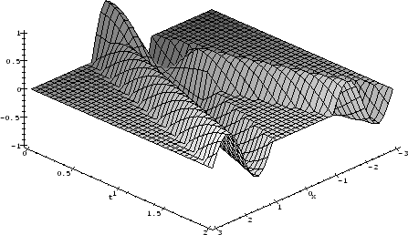
A final example:

Find the solution of

$\begin{displaymath} {1\over c^{2}}{{\partial^2 \phi}\over{\partial {t}^2}} - {{\partial^2 \phi}\over{\partial {x}^2}} = 0,\quad t>0 \end{displaymath}$

with

$\begin{displaymath} \phi(x,0) = \sin(\pi x)\hbox{ for }-1<x<1,\quad \phi(x,0) = 0\hbox{ otherwise} \end{displaymath}$

and

$\begin{displaymath} {{\partial \phi}\over{\partial x}}(x,0) = 0. \end{displaymath}$

From the above, the solution has the form

$\begin{displaymath} \phi(x,t) = {1\over 2}\left[ f(x+ct)+f(x-ct)\right] + {1\over 2c}\int^{x+ct}_{x-ct}g(y)\,dy \end{displaymath}$

where in this particular case

$\begin{displaymath} f(x) = H(1-\left\vert x\right\vert)\sin(\pi x),\quad g(x) = 0. \end{displaymath}$

Hence

$\begin{displaymath} \phi(x,t) = {1\over 2} \left[ H(1-\left\vert x-ct\right\ve... ...-\left\vert x+ct\right\vert\sin\left(\pi(x+ct)\right) \right] \end{displaymath}$

The solution is shown in the following figure:

**Figure 8.1:** Solution as a function of x and t for -3<x<3, 0<t<2
$\begin{figure} \centerline{\epsfxsize=10cm \epsffile{twave2d.ps}}\end{figure}$

Main: The Wave equation

Hosted by www.Geocities.ws