Main: The Wave equation
Waves in one space dimension
The one dimensional wave equation, with a source term, is
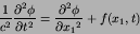 |
(44) |
We can think of this as a three dimensional equation
where, since the source term depends only on x1 and t,  depends
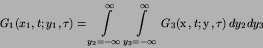
only on x1 and t. Thus the solution can be written as
depends
only on x1 and t. Thus the solution can be written as
where
 is the three dimensional Green's
function (8.3);
is the three dimensional Green's
function (8.3);
Now, since f depends only on y1 and  we can write
If we define
 by
by
 |
(45) |
then we have
so that
must be the Green's function for
(8.6), that is
This observation is known as the method of descent; we
descend from the solution of the three dimensional problem to the
solution of the one (or two) dimensional problem. It is equally valid
for the Poisson, Helmholtz and Diffusion equations, although it is
rather pointless in the case of the Diffusion equation (where we use
the one dimensional Green's function to find the three dimensional
one).
In order to find
 we have to find the integral
First we write
 and
and  to that the
problem becomes
to that the
problem becomes
where
z1=x1-y1 (and
z2=x2-y2,
z3=x3-y3, but since all of x2, x3, y2 and
y3 are going to be integrated away, this is not particularly
important). Now introduce cylindrical polar co-ordinates in which
z1 is the axial direction and
so that
z12+z22+z32 = z12+r2
and
with
 ,
,
 and
and
 .
Then
.
Then
and hence
As the integrand does not depend on  and as
this becomes
Now note that
so that
if we put
and note that when r=0
this becomes
If
 the integral is zero (since T-q is
always negative in the integral) and if
the integral is zero (since T-q is
always negative in the integral) and if
 the
integral is one (since we are integrating the delta function across a
zero of its argument
the
integral is one (since we are integrating the delta function across a
zero of its argument
 .
Thus
.
Thus
and since
z1=x1-y1,
we find that
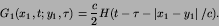 |
(46) |
Main: The Wave equation