


Next: COMPLEX RADIAL BASIS FUNCTION
Up: Adaptive Equalization of Non-linear
Previous: RADIAL BASIS FUNCTION NETWORK
RADIAL BASIS FUNCTION NETWORK AS
EQUALIZERS
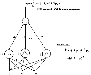
The Radial Basis Function Network (RBFN) [4] is a two layer
processing structure as shown in Figure 1. The hidden layer
consists of an array of computing nodes. Each node contains a parameter
vector called centre and the unit calculates a squared distance between
the centre and the network input vector. The squared distance is then
divided by a parameter called width and the result is passed through a
non-linear function. The second layer is a linear combiner with a set of
connection weights. The overall response of the RBF network is a mapping
fr,
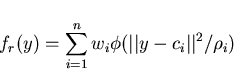 |
(1) |
where n is the number of computing nodes, ci are the RBF centres,
 are the widths of the nodes,
  is the basis function and
wi are the weights. A different type of approach is also proposed in
[7].
is the basis function and
wi are the weights. A different type of approach is also proposed in
[7].
Figure 1:
Schematic of RBF network.
 |
Comparing the network response with the optimal Bayesian
equalizer solution it has been shown [4] that both have an
identical structure. The RBF network is therefore an ideal processing
means to implement the optimal equalizer. Given channel, co-channel and
the noise statistics, it is known exactly how to specify all the
parameters of the RBF network. The number of hidden nodes n is equal to
number of noise free observation states and the RBF centres are placed at
these states. The non-linear function  is chosen as an exponential
function
is chosen as an exponential
function
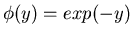 because it is a bounded and localized
function. All the widths have the same value
because it is a bounded and localized
function. All the widths have the same value
 ,
which
is twice as large as the noise variance. Each hidden node than implements
a component conditional density function and the weights are fixed
corresponding to
,
which
is twice as large as the noise variance. Each hidden node than implements
a component conditional density function and the weights are fixed
corresponding to  or
or  ,
where
is some small
constant. The RBF network then realizes precisely the optimal equalizer.
,
where
is some small
constant. The RBF network then realizes precisely the optimal equalizer.
The equalizer decision function in (1) provides a localized
behaviour. This can be modified in the normalized form to provide
non-localized behavior providing the right decision to all input vectors.
The normalized equation would be
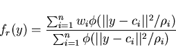 |
(2) |
The estimation of the decision function needs in (1) and
(2)
needs the channel estimation for the evaluation of the equalizer decision
function. The channel state estimation needs the channel information which
in most cases is not available. Under these circumstances the channel
states can be estimated during the training period. This can be achieved
with the help of any adaptive algorithm like LMS or RLS, but this
technique suffers failure which arises due to non-linearity. The channel
states can also be calculated directly with the help of some clustering
algorithm. The training time may be large in this but the convergence due
to this blind clustering procedure is guaranteed.
Next: COMPLEX RADIAL BASIS FUNCTION
Up: Adaptive Equalization of Non-linear
Previous: RADIAL BASIS FUNCTION NETWORK
Temp DNS admin
1999-02-03