The numerical solution of differential equations using finite element methods involves constructing a mesh of many small elements over the physical domain. On a distributed memory parallel computer, the mesh should be decomposed into subdomains, the number of which corresponds to the number of processors. The decomposition should be such that
This task of mesh decomposition is related to the graph partitioning problem, which was proved to be NP-hard. A number of graph partitioning algorithms have been suggested, among them are those based on geometric information (e.g. recursive coordinate bisection, recursive inertial bisection); algorithms based on connectivity information (e.g. recursive spectral bisection [13], greedy algorithms [3]); local and global optimisation type algorithms (e.g. Kernighan-Lin algorithm [11], simulated annealing [18]). Multilevel techniques [1] have been introduced to speed up the algorithms as well as to provide a global view of the problem. Algorithms combining the multilevel idea and the local optimisation algorithms were found to be the most successful [16,9,5]. For very large meshes (graphs) parallel algorithms are necessary [17,10,2].
Once a partition is given, each subdomain is assigned to a processor, and after some computation, processors exchange data on the shared boundaries of the subdomains. This process of computation and exchange of data goes on until the solution has converged. The data exchange is achieved by each processor sending messages to and receiving messages from processors that it shares subdomain boundaries with.
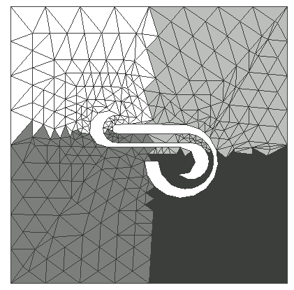
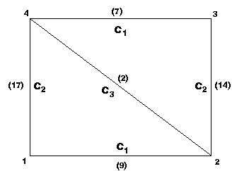
Figure 1 shows a mesh which is partitioned into 4 subdomains, assigned to processors numbered 1, 2, 3, and 4. Figure 2 shows the communication task graph of the partition. For example, processor 2 has to exchange information with processors 1, 3 and 4. The numbers in brackets in Figure 2 are the number of edges shared between processors, thus, for example, processors 2 and 4 share 2 edges. The communication task of Figure 2 can also be described by a communication task table (Table 1), in which the first column lists the identities of the processors, the other entries list the identities of adjacent processors ( adjproc) and the corresponding message lengths ( msglen, in brackets) for data exchange. Table 1 shows that processor 3 has to exchange messages with processors 2 and 4, with message lengths 14 and 7 respectively.
| Processor |
|
||
| 1 | 2(9) | 4(17) | - |
| 2 | 1(9) | 3(14) | 4(2) |
| 3 | 2(14) | 4(7) | - |
| 4 | 1(17) | 2(2) | 3(7) |
On many parallel platforms the communication time for sending a message is roughly linear in the message length, subject to a start-up cost. Therefore, for convenience and machine independence, in this paper the message length is used as an indication of the actual communication cost. However one can always replace the message length by the estimated time of sending a message of this length and all the algorithms of the paper still apply.
It is important to minimise the communication time because as more processors are used, the communication overhead becomes one of the bottlenecks for good efficiency. The problem of efficient scheduling of message passing for finite element type applications was addressed by Venkatakrishnan et al. [14]. They assumed that there were no link contentions and that the communication time between the processors was uniform. This implies that either the message lengths between processors are uniform or that the start-up time of communication dominates. They suggested that the communication can be done in a number of stages. At each stage, processors are grouped into pairs and do ``pair-wise exchange'', without interference from other processors. For example, the communication task given by the graph shown in Figure 2 can be executed in three stages as described by Table 2. In the first stage, processors (1,2) and (3,4) exchange messages. In the second stage, processors (1,4) and (2,3) exchange messages and in the final stage processors (2,4) exchange messages. In between each stage, a synchronisation is carried out.
| Processor |
|
||
| 1 | 2(9) | 4(17) | - |
| 2 | 1(9) | 3(14) | 4(2) |
| 3 | 4(7) | 2(14) | - |
| 4 | 3(7) | 1(17) | 2(2) |
A scheduling scheme which incorporates the feature that one processor is paired with at most one other processor at any stage, and that any two processors that are linked in the communication graph are paired at some stage, is equivalent to the solution of the problem of graph edge-colouring. In this problem all the edges of the graph are to be coloured such that no two edges that start from the same vertex have the same colour.
For example, the scheduling scheme given in Table 2 is equivalent
to colouring the edges between 1, 2 and 3, 4 in Figure 2 with colour
![]() , the edges between 2, 3 and 1, 4 with colour
, the edges between 2, 3 and 1, 4 with colour ![]() , and the edge between
2, 4 with colour
, and the edge between
2, 4 with colour ![]()
Let ![]() denotes the maximum number of messages to
be sent, or degree of the communication task graph
(in Figure 2
denotes the maximum number of messages to
be sent, or degree of the communication task graph
(in Figure 2 ![]() ). Venkatakrishnan et al. [14] derived a scheme that can complete
the message exchange in no more than
). Venkatakrishnan et al. [14] derived a scheme that can complete
the message exchange in no more than
![]() stages, although they did not give details of their algorithm.
stages, although they did not give details of their algorithm.
In this paper it is assumed that there are no link
contentions, but the message lengths may vary and the start-up
cost may not necessarily dominate the communication time.
Under these assumptions the total communication
time of a scheme is the sum of the longest time at each stage (plus the
synchronisation cost). For example
the communication cost of the scheduling scheme given in
Table 2 is ![]() Two scheduling schemes of the same communication task and
with the same number of stages can thus give different communication costs.
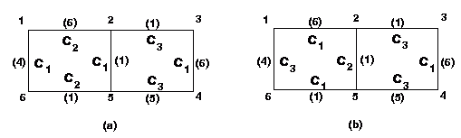
For example Figure 3 shows two schemes for the
same communication task graph. The communication time
between processors is given in brackets and three colours
Two scheduling schemes of the same communication task and
with the same number of stages can thus give different communication costs.
For example Figure 3 shows two schemes for the
same communication task graph. The communication time
between processors is given in brackets and three colours ![]() ,
, ![]() and
and ![]() ,
which correspond to three stages of the communication schemes, are used.
The first scheme (Figure 3 (a)) requires
,
which correspond to three stages of the communication schemes, are used.
The first scheme (Figure 3 (a)) requires ![]() units of time,
the second scheme
(Figure 3 (b)) needs only
units of time,
the second scheme
(Figure 3 (b)) needs only ![]() units of time.
Thus in deriving scheduling schemes,
one should also seek to minimise the sum of the largest weight of
edges with the same colour. This problem is denoted as the minimum cost
problem.
units of time.
Thus in deriving scheduling schemes,
one should also seek to minimise the sum of the largest weight of
edges with the same colour. This problem is denoted as the minimum cost
problem.
The scheduling of communication is only one example in parallel computing where the graph edge-colouring and minimum cost problems appear. There are other applications. For instance, the Kernighan-Lin (KL) algorithm [11] is usually used to reduce the number of shared edges (edge-cuts) of an initial crude partition of a graph. In the case of bisection, a gain is worked out for each vertex on the two subdomains, which represents the reduction in edge-cuts had the vertex been moved to the other subdomain. Every iteration, one vertex will be picked and moved from the subdomain with more vertices to the one with less vertices. The vertex is chosen to be the one with the largest gain. Implementing the algorithm in parallel on many processors presents a challenge, as without modification the KL algorithm is sequential in nature. One way of implementing the KL algorithm in parallel [2] is to do the refinement in a number of stages. At each stage, processors (subdomains) are grouped in pairs. Paired subdomains will refine their boundaries without interference from others. To derive such a scheduling scheme again requires solving the graph edge-colouring problem.
Furthermore, as the amount of time taken by each pair of processors in refining their boundary is usually proportional to the length of the boundary, the colouring scheme should be such that the sum of the largest length of the boundaries of each stage is minimised, this gives rise once more to the minimum cost problem.
This paper studies algorithms for the graph edge-colouring and
minimum cost problems.
In the context of synchronous
pair-wise communication, even though
the communication cost of a scheduling scheme does not necessarily
increases with the number of colours of the scheme, in practice
this is usually the case
due to the startup and synchronisation cost associated with
each stage (colour).
Therefore only colouring schemes with no more than ![]() colours
will be considered in the following.
colours
will be considered in the following.
In Section 2, the graph edge-colouring problem is looked at and
the implementation of an algorithm which produces an
edge-colouring scheme with no more that ![]() colours will be given.
Secondly, an algorithm that attempts to solve the minimum cost problem
is introduced.
colours will be given.
Secondly, an algorithm that attempts to solve the minimum cost problem
is introduced.
These algorithms will be validated in Section 3, in the context of synchronous communication, by applying them to message passing tasks resulting from partitioning of irregular meshes.
The synchronous communication scheme is only one way of organising the communication. To give a more complete view, both synchronous and asynchronous communication schemes for a parallel finite element code will be looked at and their advantages and disadvantages compared in Section 4.
Section 5 concludes the paper with further discussion.