... operadores:¹

Un conmutador se define como $[\hat A,\hat B] = \hat A\hat B - \hat B\hat A$ y las relaciones de conmutación anotadas se pueden verificar al recordar que clásicamente $\vec M = \vec r \times \vec p$ y que los operadores cuánticos equivalentes son $\hat r \rightarrow r$ y $\hat p_k \rightarrow -i\hbar {\partial \over \partial k}; k= x,y,z$

.
.
.
.
.
.
.
.
.
.
.
.
.
.
.
.
.
.
.
.
.
.
.
.
.
.
.
.
.
.

... es²

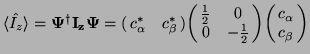
Esta definición se puede comprobar estableciendo que $\Psi^* = \langle 1\vert c_1^*+ \langle 2\vert c_2^*$ y recordando que la ortonormalidad de las funciones de base garantiza que $\langle 1\vert 1\rangle =\langle 2\vert 2\rangle =1$ y que $\langle 1\vert 2\rangle =\langle 2\vert 1\rangle =0$

.
.
.
.
.
.
.
.
.
.
.
.
.
.
.
.
.
.
.
.
.
.
.
.
.
.
.
.
.
.

... es³

En un análisis semi-cuántico, el momento magnético es proporcional al momento angular ($\vec I$) de tal forma que $\mu_z=\gamma I_z$ y también $I_z=m_j\hbar$. Las transiciones permitidas son entre niveles cuyo $\Delta m_j = \pm 1$ (regla de selección). Entonces

$$\Delta E = \hbar \gamma B_o$$

$$h \nu = h {\omega \over 2\pi} = {h \over 2\pi} \gamma B_o \rightarrow \omega=\gamma B_o$$

.
.
.
.
.
.
.
.
.
.
.
.
.
.
.
.
.
.
.
.
.
.
.
.
.
.
.
.
.
.

... resultado:⁴

$\Psi=c_\alpha \vert\alpha\rangle + c_\beta \vert\beta\rangle$. Por ejemplo, $\langle\hat{I_z}\rangle =\bf \Psi^\dagger \bf I_z\bf \Psi = \left(\matrix{ c_\a... ...r 0 & -\frac{1}{2}\cr} \right)\!\left(\matrix{ c_\alpha\cr c_\beta\cr}\right)$

.
.
.
.
.
.
.
.
.
.
.
.
.
.
.
.
.
.
.
.
.
.
.
.
.
.
.
.
.
.

... magnetizaci\'on⁵

Recordar que $e^{\pm i\theta}=\cos{\theta}\pm i\sin{\theta}$

.
.
.
.
.
.
.
.
.
.
.
.
.
.
.
.
.
.
.
.
.
.
.
.
.
.
.
.
.
.

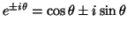
... anterior⁶

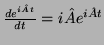
Se emplean las siguientes propiedades:

$$\langle \phi\vert\hat{A}\psi\rangle =\langle\hat{A}^\dagger\p... ...t\psi\rangle ; \hat{A}^\dagger\hat{A}=\hat{A}\hat{A}^\dagger=1$$

.
.
.
.
.
.
.
.
.
.
.
.
.
.
.
.
.
.
.
.
.
.
.
.
.
.
.
.
.
.

... anterior⁷

$\frac{de^{i\hat{A}t}}{dt} = i\hat{A}e^{i\hat{A}t}$

.
.
.
.
.
.
.
.
.
.
.
.
.
.
.
.
.
.
.
.
.
.
.
.
.
.
.
.
.
.

... forma⁸

La justificación del resultado es la siguiente: La ecuación de LN es

$$\frac{d\hat{\rho}}{dt}=-ib[\hat{B},\hat{\rho}]$$

$$-ib[\hat{B},\hat{A}]=ib[\hat{B},(\hat{A}\cos{(bt)}-\hat{C}\si... ...at{B},\hat{C}]\sin{(bt)}=-b\hat{C}\cos{(bt)}-b\hat{A}\sin{(bt)}$$

Que es lo mismo que se obtiene al derivar a (27)

$$\frac{d\hat{\rho}(t)}{dt}=-ib(-i\hat{C})\cos{(bt)}+ib(i\hat{A})\sin{(bt)}$$

$$=-b\hat{C}\cos{(bt)}-b\hat{A}\sin{(bt)}$$

.
.
.
.
.
.
.
.
.
.
.
.
.
.
.
.
.
.
.
.
.
.
.
.
.
.
.
.
.
.

Hosted by www.Geocities.ws