Chemistry
First Order Kinetics
Beginning chemistry students often find themselves confused learning the governing laws of kinetics. It is imperative for an instructor to relate mathematical concepts to the physical meaning of terms. The following is an attempt to describe first-order kinetics in an intuitive way.
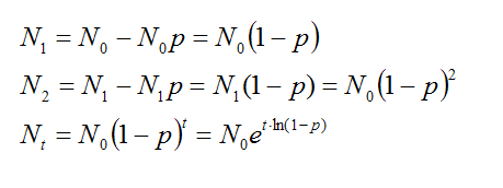
The key to understanding first order kinetics is to realize that the amount of reactant at any given time depends upon the amount of reactant at previous time. It is also important to develop a sense of infinitesimal time scale and imagine that chemical reactions occur on that scale. At a given instance in time, the amount of reactant equals to the amount at previous time minus the probability of reaction occurring multiplied by the amount of reactant at previous time. Below is the mathematical representation of this statement.
Similar approach is used to
analyze bimolecular reactions: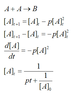
The result above requires knowledge of calculus.
Simulating the Law of Mass Action
The law of mass action, or the rate law, says that
the rate of a chemical reaction is proportional to the concentrations of
reactants. Considering the simple reaction below:
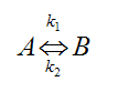
The rate of the forward reaction is proportional to the concentration of A and k1
and the rate of reverse reaction to the concentration of B and k2.
Most general chemistry textbooks do not show the derivation of the rate law due
to the amount of material that needs to be absorbed by the beginners. The
explanation below should satisfy mathematically oriented student.
Essentially Brownian motion leads to molecular collisions which allow overcoming activation energy barriers. For the purposes of this simulation, the space of molecular motion is assumed to consist of 100 positions. The program creates an array N of 100 integer values. Each element of the array represents a position in 3-dimensional space. Each element can have any integer value greater than 0. The value denotes the number of molecules of A in that position at a given point in time.
The program simulates molecular
motion by adding molecules to one position and subtracting them from the other.
On each iteration, a random number generator gives two values: position of one
molecule (p1) and position of the other (p2). Next, the
program decrements the Np1 and increments Np2. As a result
of repeating this cycle several hundred times, molecules achieve random
distribution and the Brownian motion of the molecules is simulated.
After one round of rearrangement, the program scans N and detects all the
elements that have values greater than 1. These positions contain more than one
molecule A at that moment in time. This is equivalent to a molecular collision
and, therefore, the value of N at that position is decremented (one molecule of
A is transformed to B). The total number of molecules transformed from A to B is
recorded on each iteration and is plotted against the time on the graph. This
plot is reminiscent of the plot of the concentration of A versus time that is
usually drawn to the students in general chemistry textbooks.
Proving the Law of Chemical Equilibrium Using Series Convergence
It is often taken for granted by the beginning chemistry students that there exists a state of chemical equilibrium in which both forward and reverse reactions proceed at the same rate. Occasionally, a keen student may ask the following question: is it possible to show mathematically that the state of equilibrium can be reached? This article explains just how it can be done.
For the situation shown above, the time course of the reaction is divided into discrete steps. In the first step, A loses part of its concentration and that part is added to B. In the second step, B loses part of its concentration and A gains that part.
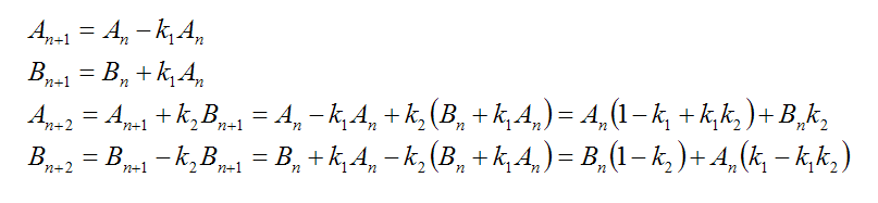
In essence, the existence of chemical equilibrium should be proved if we prove that A and B converge as n approaches infinity. In order to prove convergence, one has to be familiar with linear algebra. The matrix below describes the changes in concentrations of A and B at the end of one iteration:
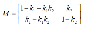
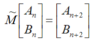
If we could prove that n-th power of M transforms initial concentrations in accord with equilibrium principle, then we would prove equilibrium mathematically.
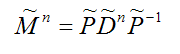
In order to raise matrix to n-th power, we diagonalize it with matrix P such that columns of P are eigenvectors of M
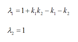
The eigenvalues of M are given below
and this is the P matrix
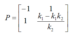
The inverse of P is given below

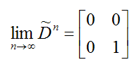
Since we are interested in the limit of D as n approaches infinity, we need only to realize that eigenvalue of 1 will remain 1 in the limit whereas the other eigenvalue will become negligibly small. Thus we take the value of D to be as below:
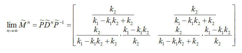
And the limit of n-th power of M is
If we transform initial concentration values with the matrix above, we will have:
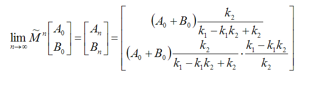
In the limit, the ratio of B to A will be as below
which is very close to the equilibrium constant. This solution was influenced by answer from Dr. Robert Israel.
Entropy
Why does the transfer of heat and equilibration of
temperature between two bodies increases the entropy? High temperature means
higher kinetic energy for the molecules in the closed system. As a result, the
molecules will have a higher probability of occupying any given position in
space. Therefore, higher temperature can be thought of as higher number of
positions in space available for the molecules.
Suppose closed system A has higher temperature than B. For the sake of
simplicity, let A have six total available positions for its molecules and let B
have four. Suppose we have total of two molecules occupying each system. First
molecule in system A can take six possible positions and the second molecule
will be left with five. Thus the total number of possible arrangements within
system A is 30. By analogy, the second system will have 12 possible arrangements
of molecules. In order to describe the total number of possible states available
for both A and B, we multiply 30 by 12 which gives 360. Now, let's suppose both
A and B attained thermal equilibrium and their final temperature allows their
molecules to occupy five possible positions in each system. Now, two molecules
in A can occupy 20 possible states and so is true about molecules in B. The
total number of possible states for both A and B is now 400. Therefore, upon
reaching thermal equilibrium, the total number of states available for both
systems has increased, confirming the second law of thermodynamics.
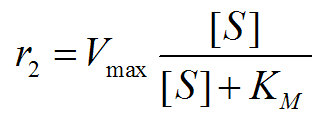
Michaelis-Menten Kinetics
The most useful model that describes enzyme catalyzed reactions is Michaelis-Menten steady-state kinetics. The reaction mechanism can be written as below:
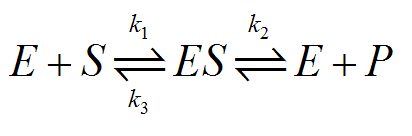
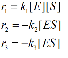
Here E stands for enzyme, S stands for substrate, ES is enzyme-substrate complex and P is the product. Notice that at the start of the reaction, the concentration of the product is not significant enough to cause reverse reaction at the second step so we omit k4. The idea of steady-state kinetics is that at a certain point, the rate of enzyme-substrate complex formation is equal to the rate of its dissociation. Let's write down equations for the rates of the reactions that are depicted in this equation:
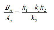
The key equation of the Michaelis-Menten theory is written below:
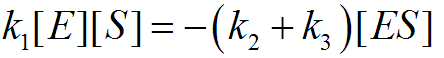
It is important to realize that the concentration of free enzyme is equal to the difference of enzyme-substrate and free substrate concentrations, thus the substitution made below is justified:
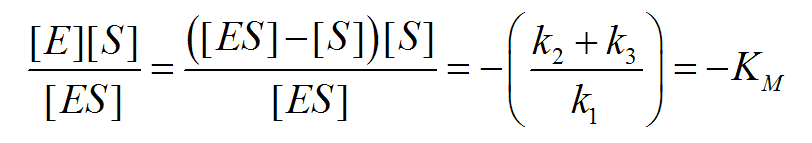
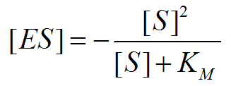
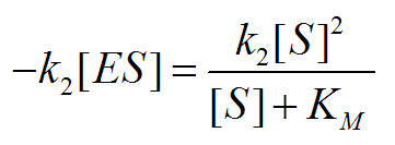
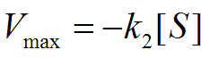
Solving for [ES], we obtain the following equation:
A Java applet simulating kinetics of Michaelis-Menten model is here.