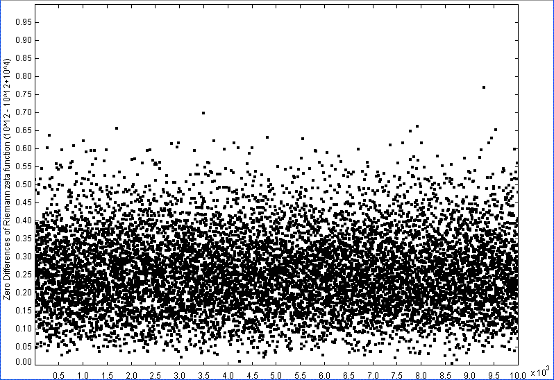
We studied the fractal structure of the Riemann zeta zeros using
Rescaled Range Analysis.
The self-similarity of the zero distributions is quite remarkable,
and is characterized by a large fractal dimension of 1.9 (equivalently,
a Hurst Exponent of 0.1). The differences of the zeros are shown
in the figure below.
Not only is the fractal dimension unusually high, it is also surprisingly
constant, even when calculated
over fifteen orders of magnitude for the Riemann function.
The very striking behaviour for the zeros of the Riemann zeta function is also shared by other L functions. The table shows the calculation for the L-functions. In the table, r indicates an index to which of the group character representations is being considered for the L-function.
| Order of | Hurst | Fractal | |
|---|---|---|---|
| largest zero | exponent | Dimension | |
| Riemann Zeta | |||
| 35161820 | 0.091 | 1.909 | |
| 10^12 | 0.093 | 1.907 | |
| 10^21 | 0.094 | 1.906 | |
| 10^22 | 0.100 | 1.900 | |
| Degree 1 L-function, Conductor 3 | |||
| 31712310 | 0.092 | 1.908 | |
| Degree 1 L-function, Conductor 4 | |||
| 32457680 | 0.092 | 1.908 | |
| Degree 1 L-function, Conductor 9 | |||
| Dirichlet Character | |||
| 10000000 | r=2 conjugate pair, negative roots | 0.094 | 1.906 |
| 10000000 | r=2 conjugate pair, positive roots | 0.097 | 1.903 |
| 10000000 | r=3 conjugate pair, negative roots | 0.114 | 1.886 |
| 10000000 | r=3 conjugate pair, positive roots | 0.084 | 1.916 |
| Degree 1 L-function, Conductor 19 | |||
| Dirichlet Character | |||
| 1000000 | r=2 conjugate pair, negative roots | 0.105 | 1.895 |
| 1000000 | r=2 conjugate pair, positive roots | 0.116 | 1.884 |
| 1000000 | r=3 conjugate pair, negative roots | 0.123 | 1.877 |
| 1000000 | r=3 conjugate pair, positive roots | 0.103 | 1.897 |
| 1000000 | r=4 conjugate pair, negative roots | 0.096 | 1.904 |
| 1000000 | r=4 conjugate pair, positive roots | 0.112 | 1.888 |
| 1000000 | r=5 conjugate pair, negative roots | 0.094 | 1.906 |
| 1000000 | r=5 conjugate pair, positive roots | 0.105 | 1.895 |
| 1000000 | r=6 conjugate pair, negative roots | 0.125 | 1.875 |
| 1000000 | r=6 conjugate pair, positive roots | 0.099 | 1.901 |
| 1000000 | r=7 conjugate pair, negative roots | 0.100 | 1.900 |
| 1000000 | r=7 conjugate pair, positive roots | 0.106 | 1.894 |
| 1000000 | r=8 conjugate pair, negative roots | 0.116 | 1.884 |
| 1000000 | r=8 conjugate pair, positive roots | 0.104 | 1.896 |
| 1000000 | r=9 conjugate pair, negative roots | 0.098 | 1.902 |
| 1000000 | r=9 conjugate pair, positive roots | 0.121 | 1.879 |
| 1000000 | r=10 real representation, positive roots | 0.089 | 1.911 |
| Degree 2 Elliptic curve L-function, Conductor 19 isogeny class A | |||
| 100000 | 0.091 | 1.909 | |
| Degree 2 L-function, Ramanujan tau (associated cusp form of weight 12, level 1) | |||
| 284410 | 0.108 | 1.892 | |
We compared the behaviour of the Riemann zeros with
that of the Random Matrix Theories, which explain many properties
of the Riemann zeroes. For the Hurst exponents the
Random Matrix results seem to differ from the Riemann zero results.
However, this statement has to be treated with caution, since the
sample sizes considered for the two systems differ significantly.
The low Hurst exponent seems to be connected with the relation
between the Riemann zeroes and the prime numbers, as explained
in my paper. The role of the primes in statistics of the zeta zeros is
closely related to the behaviour of quantum chaotic systems.
Berry
has several introductory articles on quantum chaos, including applications
to the Riemann zeta function.
It is well-known that there are
certain statistics
connected with the Riemann zeta function that are "universal" if one
studies the zeta
function, or its zeros, high on the critical line. That is, in the limit
of large height
up the critical line, these "local" statistics follow predictions from
random matrix theory.
Then there are other
statistics, such as the distribution of values of the zeta function
itself, that depend
on zeros over much larger ranges, and therefore take into account
longer-range correlations
between the zeros. These do not show universal behaviour. In fact,
this type of
statistic has crucial dependence on the prime numbers, exactly as
we find for the
Hurst exponent. In many cases very
precise expressions can
be written down showing explicitly the contributions from the primes, so
in fact we know
rather a lot about the role primes play in zero statistics.
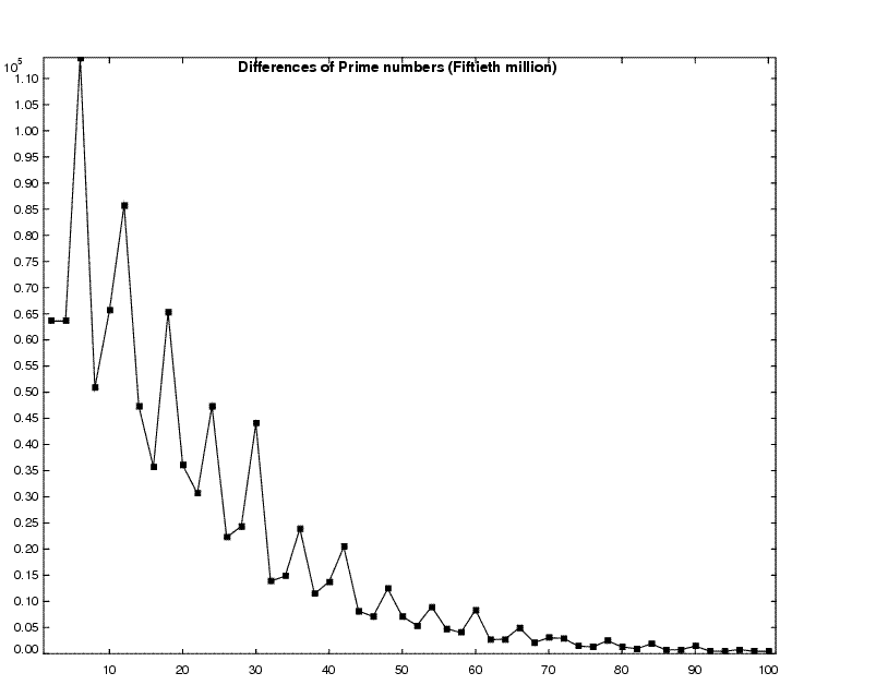
Since the Riemann zeta zeros are related to the distribution of
prime numbers, we study the distribution.
The distribution for the differences of the prime numbers is shown
in the figure below for the fiftieth million set of primes.
The horizontal axis shows the difference between consecutive primes,
and the vertical axis shows the count for the number of times the
difference occurs in the fiftieth million set of primes.
The structure in the histogram is interesting, e.g., the peaks when the
differences are multiples of 6. When a prime number is divided by 6,
the remainder is either 1 or 5. An analysis of the peaks gives
information on the correlation between
the probability of the remainder being 1 or 5 and the
remainder for the previous prime number.
From the histogram, we get the following probabilities:
Prob(diff=6k+2) = Prob(diff=6k+4) = .276;
Prob(diff=6k) = 0.448;
If there were no correlations between neighbouring primes, then the values would be closer to
Prob(diff=6k+2) = Prob(diff=6k+4) = .25;
Prob(diff=6k) = 0.50;
Are we seeing signs of a correlation between neighbouring primes here?
If so, it would be very exciting. A closer look at the prime number
statistics seems warranted.
See Distribution of Primes and
Rescaled Range Analysis of L-function zeros and Prime Number distribution.
I have used the zeroes from
http://www.dtc.umn.edu/~odlyzko/zeta_tables/index.html and
http://pmmac03.math.uwaterloo.ca/~mrubinst/L_function_public/ZEROS/.
For the serious investigator into number theory, the
Number Theory Web gives
a good number of links. You may also wish to visit the interesting sites of Watkins
on fractality in number theory and
Number Theory and Physics. The sites provide many links to work related to what I have done, and I encourage you to look into the papers.
Here are a couple of sites which explain the
Hurst Exponent and
Rescaled Range analysis. Zeta functions also arise in a variety of other contexts.
For example, one can define
graph zeta functions
which may be applied to
study the dimension of a complex network (large network of nodes connected
by edges).
G J Chaitin has
talked about
experimental mathematics, and it is amusing that the work that I have done falls right into the
kind of thing he has been mentioning!
Here are links to: my home page, and O. Shanker publication list.