Spherically symmetric collapsar in the relativistic theory of gravitation
Vladimir L. Kalashnikov
TU Wien, Gusshausstr. 27/387, A-1040 Vienna, Austria
tel: +43-1-58801-38723 , fax: +43-1-58801-38799
The relativistic theory of gravitation (RTG) differs from Einstein's theory of the general relativity (GR) in the crucial point: it refutes the total geometrization and considers the gravitation as a manifestation of the two-rank tensor field embedded in the flat Minkowski's background space-time. The universality of gravitation manifests itself through appearance of the effective curved Riemannian space-time governing the matter motion. The source of the curvature of the effective space-time is the energy-momentum tensor of the matter. Unlike the GR there is the unique one-to-one correspondence between Minkowski's and Riemannian's coordinates so the background metric can be restored in any situation. This is possible due to an insertion of the Minkowski's metric into structure of the field Lagarngian. This results in the violation of the gauge-invariance and in the appearance of the non-zero graviton mass.
Among the remarkable physical consequences of the RTG there are i) absence of the cosmological singularity due to antigravitation caused by the massive graviton; ii) flat effective cosmological space-time resulted from the field equations; iii) impossibility of the black holes. Topics i) and ii) are considered in rtg.html, topic iii) will be considered in this worksheet.
Note, that the evaluation of this worksheet takes about of 20 min (Athlon XP2600+) and 34 Mb of RAM.
REFERENCES:
A.A.Logunov, "The theory of gravity"
Spherically symmetric metric
The general spherically symmetric static metric can be introduced in the following way:
| > | restart: with(tensor): with(linalg): with(DEtools): with(plots): with(stats): coord := [t, r, theta, phi]:# spherical coordinates g_compts := array(symmetric,sparse,1..4,1..4): g_compts[1,1] := U(r):#dt^2 g_compts[2,2] := - V(r):#dr^2 g_compts[3,3] := -W(r)^2:#dtheta^2 g_compts[4,4] := -W(r)^2*sin(theta)^2:#dphi^2 g := create([-1,-1], eval(g_compts));# covariant components of metric ginv := invert( g, 'detg' );# contravariant components of metric g_scal := det(get_compts(g));# scalar of the metric tensor |
Warning, the protected names norm and trace have been redefined and unprotected
Warning, the name adjoint has been redefined
Warning, the name changecoords has been redefined
Warning, the name transform has been redefined
![g := TABLE([index_char = [-1, -1], compts = matrix([[U(r), 0, 0, 0], [0, -V(r), 0, 0], [0, 0, -W(r)^2, 0], [0, 0, 0, -W(r)^2*sin(theta)^2]])])](images/rtg_bh1.gif)
![ginv := TABLE([index_char = [1, 1], compts = matrix([[1/U(r), 0, 0, 0], [0, -1/V(r), 0, 0], [0, 0, -1/(W(r)^2), 0], [0, 0, 0, -1/(W(r)^2*sin(theta)^2)]])])](images/rtg_bh2.gif)
![]()
The density of the metric tensor
![]()
![]() is
is
| > | gg_compts := array(symmetric,sparse,1..4,1..4): gg_compts[1,1] := simplify( sqrt( -g_scal )*get_compts(ginv)[1,1],symbolic,radical ):#dt^2 gg_compts[1,2] := simplify( sqrt( -g_scal )*get_compts(ginv)[1,2],symbolic,radical ):#dt*dr gg_compts[2,2] := simplify( sqrt( -g_scal )*get_compts(ginv)[2,2],symbolic,radical ):#dr^2 gg_compts[3,3] := simplify( sqrt( -g_scal )*get_compts(ginv)[3,3],symbolic,radical ):#dtheta^2 gg_compts[4,4] := simplify( sqrt( -g_scal )*get_compts(ginv)[4,4],symbolic,radical ):#dphi^2 `g*` := create([1,1], eval(gg_compts)); |
![]()
![`g*` := TABLE([index_char = [1, 1], compts = matrix([[(U(r)*V(r)*W(r)^4*sin(theta)^2)^(1/2)/U(r), 0, 0, 0], [0, -(U(r)*V(r)*W(r)^4*sin(theta)^2)^(1/2)/V(r), 0, 0], [0, 0, -(U(r)*V(r)*W(r)^4*sin(theta)^...](images/rtg_bh7.gif)
![]()
The background Minkowski's metric
![]() in the spherical coordinates is
in the spherical coordinates is
| > | mu_compts := array(symmetric,sparse,1..4,1..4): mu_compts[1,1] := 1:#dt^2 mu_compts[2,2] := -1:#dr^2 mu_compts[3,3]:= -r^2:#dtheta^2 mu_compts[4,4]:= -r^2*sin(theta)^2:#dphi^2 mu := create([-1,-1], eval(mu_compts));# covariant components of mu muinv := invert( mu, 'detg' ): |
![mu := TABLE([index_char = [-1, -1], compts = matrix([[1, 0, 0, 0], [0, -1, 0, 0], [0, 0, -r^2, 0], [0, 0, 0, -r^2*sin(theta)^2]])])](images/rtg_bh10.gif)
The first field equation is
![D[m]*`g*`^mn = 0](images/rtg_bh11.gif) (
(
![]() is the covariant derivative on the background metric). This equation eliminates the undesirable spin states for the graviton.
is the covariant derivative on the background metric). This equation eliminates the undesirable spin states for the graviton.
| > | # the covariant derivative on the background metric A1 := partial_diff( `g*`, coord ): A2 := contract(A1,[2,3]): d1mu:= d1metric(mu, coord): Cf1:= Christoffel1 ( d1mu ): Cf2:= Christoffel2 ( muinv, Cf1 ): ZZZ := prod(Cf2,`g*`): A3 := contract(ZZZ,[2,5] ): A4 := contract(A3,[2,3]): simplify(get_compts(A2)[1] + get_compts(A4)[1]); e1 := simplify(get_compts(A2)[2] + get_compts(A4)[2]); simplify(get_compts(A2)[3] + get_compts(A4)[3]); |
![]()
![]()
![]()
![]()
![]()
The obtained equation is:
| > | factor( numer( e1 ) ): e2 := expand( %/(W(r)^2*(cos(theta)-1)*(cos(theta)+1)) ); |
![]()
Which results in:
| > | eq[1] := Diff( sqrt(U(r)/V(r))*W(r)^2,r) = 2*r*sqrt(V(r)*U(r)) ; print(`check-up:`); factor(numer( simplify( simplify( value(lhs(eq[1])) - rhs(eq[1]))) ) - e2 ); |
![]()
![]()
![]()
Now let's consider the energy-momentum tensor.
| > | T_compts := array(symmetric,sparse,1..4,1..4):# energy-momentum tensor components T_compts[1,1] := U(r)*rho(r): T_compts[2,2] := V(r)*p(r): T_compts[3,3] := W(r)^2*p(r): T_compts[4,4] := W(r)^2*sin(theta)^2*p(r): T := create([-1,-1], eval(T_compts));# covariant energy-momentum tensor |
![T := TABLE([index_char = [-1, -1], compts = matrix([[U(r)*rho(r), 0, 0, 0], [0, V(r)*p(r), 0, 0], [0, 0, W(r)^2*p(r), 0], [0, 0, 0, W(r)^2*sin(theta)^2*p(r)]])])](images/rtg_bh22.gif)
| > | # mixed energy-momentum tensor macro(Ts=`T*`): T_compts := array(symmetric,sparse,1..4,1..4):# energy-momentum tensor components T_compts[1,1] := rho(r): T_compts[2,2] := -p(r): T_compts[3,3] := -p(r): T_compts[4,4] := -p(r): Ts := create([-1,1], eval(T_compts));# [-1,1] energy-momentum tensor |
![`T*` := TABLE([index_char = [-1, 1], compts = matrix([[rho(r), 0, 0, 0], [0, -p(r), 0, 0], [0, 0, -p(r), 0], [0, 0, 0, -p(r)]])])](images/rtg_bh23.gif)
The covariant conservation law is
![]() [;
n
]= 0, where [;
n
] denotes the covariant derivative on the Riemannian metric.
[;
n
]= 0, where [;
n
] denotes the covariant derivative on the Riemannian metric.
| > | d1g:= d1metric(g, coord):# covariant derivative Cf1:= Christoffel1 ( d1g ): Cf2:= Christoffel2 ( ginv, Cf1 ): Z := cov_diff( Ts, coord, Cf2 ): ZZ := contract(Z,[2,3]); |
![ZZ := TABLE([index_char = [-1], compts = vector([0, -1/2*(diff(U(r),r)*p(r)+diff(U(r),r)*rho(r)+2*diff(p(r),r)*U(r))/U(r), 0, 0])])](images/rtg_bh25.gif)
The resulting equation is (in addition to that obtained from the first field equation):
| > | get_compts( ZZ )[2]: numer(%): expand(%/U(r)/2) = 0; |
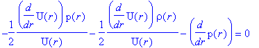
| > | eq[2] := diff(p(r),r) = -(rho(r) + p(r))*(diff(U(r),r)/2/U(r)); |
![eq[2] := diff(p(r),r) = -1/2*diff(U(r),r)*(p(r)+rho(r))/U(r)](images/rtg_bh27.gif)
Now we have to turn to the main field equation
![R[n]^m-delta[n]^m*R/2-m^2*(delta[n]^m+g^mk*mu[kn]-delta[n]^m*g^pk*mu[pk]/2)/2 = -8*pi*T[n]^m](images/rtg_bh28.gif) .
.
| > | # construction of the Einstein's tensor D1g := d1metric ( g, coord ): D2g := d2metric ( D1g, coord ): Cf1 := Christoffel1 ( D1g ): RMN := Riemann( ginv, D2g, Cf1 ): RICCI := Ricci( ginv, RMN ):# Ricci tensor RS := Ricciscalar( ginv, RICCI ):# Ricci scalar Estn := raise(ginv, Einstein( g, RICCI, RS ), 2 );# Einstein's tensor with mixed indexes |
![]()
![]()
![Estn := TABLE([index_char = [-1, 1], compts = matrix([[(2*W(r)*diff(W(r),`$`(r,2))*V(r)-diff(V(r),r)*W(r)*diff(W(r),r)-V(r)^2+V(r)*diff(W(r),r)^2)/W(r)^2/V(r)^2, 0, 0, 0], [0, -1/V(r)/U(r)*(-diff(U(r),...](images/rtg_bh31.gif)
![Estn := TABLE([index_char = [-1, 1], compts = matrix([[(2*W(r)*diff(W(r),`$`(r,2))*V(r)-diff(V(r),r)*W(r)*diff(W(r),r)-V(r)^2+V(r)*diff(W(r),r)^2)/W(r)^2/V(r)^2, 0, 0, 0], [0, -1/V(r)/U(r)*(-diff(U(r),...](images/rtg_bh32.gif)
![Estn := TABLE([index_char = [-1, 1], compts = matrix([[(2*W(r)*diff(W(r),`$`(r,2))*V(r)-diff(V(r),r)*W(r)*diff(W(r),r)-V(r)^2+V(r)*diff(W(r),r)^2)/W(r)^2/V(r)^2, 0, 0, 0], [0, -1/V(r)/U(r)*(-diff(U(r),...](images/rtg_bh33.gif)
![Estn := TABLE([index_char = [-1, 1], compts = matrix([[(2*W(r)*diff(W(r),`$`(r,2))*V(r)-diff(V(r),r)*W(r)*diff(W(r),r)-V(r)^2+V(r)*diff(W(r),r)^2)/W(r)^2/V(r)^2, 0, 0, 0], [0, -1/V(r)/U(r)*(-diff(U(r),...](images/rtg_bh34.gif)
![Estn := TABLE([index_char = [-1, 1], compts = matrix([[(2*W(r)*diff(W(r),`$`(r,2))*V(r)-diff(V(r),r)*W(r)*diff(W(r),r)-V(r)^2+V(r)*diff(W(r),r)^2)/W(r)^2/V(r)^2, 0, 0, 0], [0, -1/V(r)/U(r)*(-diff(U(r),...](images/rtg_bh35.gif)
![Estn := TABLE([index_char = [-1, 1], compts = matrix([[(2*W(r)*diff(W(r),`$`(r,2))*V(r)-diff(V(r),r)*W(r)*diff(W(r),r)-V(r)^2+V(r)*diff(W(r),r)^2)/W(r)^2/V(r)^2, 0, 0, 0], [0, -1/V(r)/U(r)*(-diff(U(r),...](images/rtg_bh36.gif)
![]()
| > | # massive term in the Logunov's equations K_compts := array(symmetric,sparse,1..4,1..4): K_compts[1,1] := 1: K_compts[2,2] := 1: K_compts[3,3]:= 1: K_compts[4,4]:= 1: K := create([-1,1], eval(K_compts)):# Kronecker symbol Z := prod(ginv,mu): term2 := contract(Z,[2,3]):# second term in brackets (field equation) ZZ := contract(Z,[2,4]): prod(K,contract(ZZ,[1,2])): term3 := prod(table([index_char = [], compts = -1/2]),%):# third term in brackets Lgv_compts := array(symmetric,sparse,1..4,1..4); Lgv_compts[1,1] := simplify( get_compts(Estn)[1,1] - ( m^2/2 )*( get_compts(K)[1,1] + get_compts(term2)[1,1] + get_compts(term3)[1,1] ) ): Lgv_compts[2,2] := simplify( get_compts(Estn)[2,2] - ( m^2/2 )*( get_compts(K)[2,2] + get_compts(term2)[2,2] + get_compts(term3)[2,2] ) ): Lgv_compts[3,3] := simplify( get_compts(Estn)[3,3] - ( m^2/2 )*( get_compts(K)[3,3] + get_compts(term2)[3,3] + get_compts(term3)[3,3] ) ): Lgv_compts[4,4] := simplify( get_compts(Estn)[4,4] - ( m^2/2 )*( get_compts(K)[4,4] + get_compts(term2)[4,4] + get_compts(term3)[4,4] ) ): Lgv := act(expand,create([-1,1], eval(Lgv_compts)));# left-hand side of "massive" field equation |
![]()
![]()
![]()
![Lgv := TABLE([index_char = [-1, 1], compts = matrix([[2/W(r)/V(r)*diff(W(r),`$`(r,2))-1/W(r)/V(r)^2*diff(V(r),r)*diff(W(r),r)-1/(W(r)^2)+1/W(r)^2/V(r)*diff(W(r),r)^2-1/2*m^2-1/4*1/U(r)*m^2+1/4*1/V(r)*m...](images/rtg_bh41.gif)
![Lgv := TABLE([index_char = [-1, 1], compts = matrix([[2/W(r)/V(r)*diff(W(r),`$`(r,2))-1/W(r)/V(r)^2*diff(V(r),r)*diff(W(r),r)-1/(W(r)^2)+1/W(r)^2/V(r)*diff(W(r),r)^2-1/2*m^2-1/4*1/U(r)*m^2+1/4*1/V(r)*m...](images/rtg_bh42.gif)
![Lgv := TABLE([index_char = [-1, 1], compts = matrix([[2/W(r)/V(r)*diff(W(r),`$`(r,2))-1/W(r)/V(r)^2*diff(V(r),r)*diff(W(r),r)-1/(W(r)^2)+1/W(r)^2/V(r)*diff(W(r),r)^2-1/2*m^2-1/4*1/U(r)*m^2+1/4*1/V(r)*m...](images/rtg_bh43.gif)
![Lgv := TABLE([index_char = [-1, 1], compts = matrix([[2/W(r)/V(r)*diff(W(r),`$`(r,2))-1/W(r)/V(r)^2*diff(V(r),r)*diff(W(r),r)-1/(W(r)^2)+1/W(r)^2/V(r)*diff(W(r),r)^2-1/2*m^2-1/4*1/U(r)*m^2+1/4*1/V(r)*m...](images/rtg_bh44.gif)
![Lgv := TABLE([index_char = [-1, 1], compts = matrix([[2/W(r)/V(r)*diff(W(r),`$`(r,2))-1/W(r)/V(r)^2*diff(V(r),r)*diff(W(r),r)-1/(W(r)^2)+1/W(r)^2/V(r)*diff(W(r),r)^2-1/2*m^2-1/4*1/U(r)*m^2+1/4*1/V(r)*m...](images/rtg_bh45.gif)
![Lgv := TABLE([index_char = [-1, 1], compts = matrix([[2/W(r)/V(r)*diff(W(r),`$`(r,2))-1/W(r)/V(r)^2*diff(V(r),r)*diff(W(r),r)-1/(W(r)^2)+1/W(r)^2/V(r)*diff(W(r),r)^2-1/2*m^2-1/4*1/U(r)*m^2+1/4*1/V(r)*m...](images/rtg_bh46.gif)
![]()
The resulting equations are:
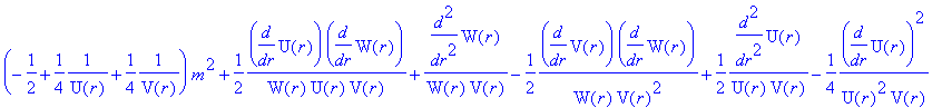
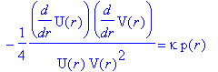
| > | eq[3] := collect( get_compts(Lgv)[1,1],m^2 ) = -kappa*get_compts(Ts)[1,1];# kappa = 8*Pi*G/c^2 |
![eq[3] := (-1/2-1/4*1/U(r)+1/4*1/V(r)+1/2*1/W(r)^2*r^2)*m^2+2/W(r)/V(r)*diff(W(r),`$`(r,2))-1/W(r)/V(r)^2*diff(V(r),r)*diff(W(r),r)-1/(W(r)^2)+1/W(r)^2/V(r)*diff(W(r),r)^2 = -kappa*rho(r)](images/rtg_bh48.gif)
| > | eq[4] := collect( get_compts(Lgv)[2,2],m^2 ) = -kappa*get_compts(Ts)[2,2]; |
![eq[4] := (-1/2-1/4*1/V(r)+1/4*1/U(r)+1/2*1/W(r)^2*r^2)*m^2+1/W(r)/U(r)/V(r)*diff(U(r),r)*diff(W(r),r)-1/(W(r)^2)+1/W(r)^2/V(r)*diff(W(r),r)^2 = kappa*p(r)](images/rtg_bh49.gif)
| > | collect( get_compts(Lgv)[3,3],m^2 ) = -kappa*get_compts(Ts)[3,3]; eq[5] := collect( get_compts(Lgv)[4,4],m^2 ) = -kappa*get_compts(Ts)[4,4]; |
![eq[5] := (-1/2+1/4*1/U(r)+1/4*1/V(r))*m^2+1/2*1/W(r)/U(r)/V(r)*diff(U(r),r)*diff(W(r),r)+1/W(r)/V(r)*diff(W(r),`$`(r,2))-1/2*1/W(r)/V(r)^2*diff(V(r),r)*diff(W(r),r)+1/2*1/U(r)/V(r)*diff(U(r),`$`(r,2))-...](images/rtg_bh52.gif)
![eq[5] := (-1/2+1/4*1/U(r)+1/4*1/V(r))*m^2+1/2*1/W(r)/U(r)/V(r)*diff(U(r),r)*diff(W(r),r)+1/W(r)/V(r)*diff(W(r),`$`(r,2))-1/2*1/W(r)/V(r)^2*diff(V(r),r)*diff(W(r),r)+1/2*1/U(r)/V(r)*diff(U(r),`$`(r,2))-...](images/rtg_bh53.gif)
Let's make some simplifications with the obtained equations.
| > | eq[3]; |
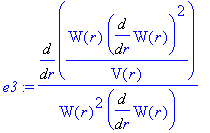
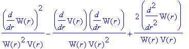
| > | e3 := Diff( ( W(r)/V(r) )*(Diff( W(r),r ))^2,r )/( W(r)^2*Diff(W(r),r)); expand( value(%) ); |
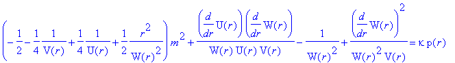
| > | eq[6] := expand( e3*W(r)^2 ) - 1 + (m^2/2)*(r^2 - W(r)^2 + W(r)^2*(1/V(r)-1/U(r))/2 ) = -kappa*rho(r)*W(r)^2; |
![eq[6] := Diff(W(r)/V(r)*Diff(W(r),r)^2,r)/Diff(W(r),r)-1+1/2*m^2*(r^2-W(r)^2+1/2*W(r)^2*(1/V(r)-1/U(r))) = -kappa*rho(r)*W(r)^2](images/rtg_bh57.gif)
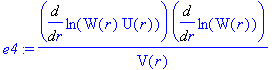
| > | eq[4]; e4 := Diff( ln(W(r)*U(r)),r)/V(r)*Diff(ln(W(r)),r); expand( value(e4) ); |
| > | eq[7] := expand( e4*W(r)^2 ) - 1 + (m^2/2)*(r^2 - W(r)^2 + W(r)^2*(1/U(r)-1/V(r))/2 ) = kappa*p(r)*W(r)^2; |
![eq[7] := Diff(ln(W(r)*U(r)),r)/V(r)*Diff(ln(W(r)),r)*W(r)^2-1+1/2*m^2*(r^2-W(r)^2+1/2*W(r)^2*(1/U(r)-1/V(r))) = kappa*p(r)*W(r)^2](images/rtg_bh61.gif)
So, we have the system of the master equations (we use the following normalizations
 ,
,
 ,
,
 ,
M
is the mass producing the spherical metric):
,
M
is the mass producing the spherical metric):
| > | # x and y are r and W, respectively, normalized to the Schwarzschild radius #l = 2*G*M/c^2; epsilon = (1/2)*(2*G*M*m/(c*(h/(2*Pi))))^2, xi=kappa*l^2 fun[1] := Diff( (x/V)/Diff(y,x)^2,x ) + subs( {r=y,m^2=2*epsilon,W(r)=x,V(r)=V,U(r)=U},lhs(eq[6]) - op(1,lhs(eq[6])) ) = subs( {kappa=xi,rho(r)=rho(x),W(r)=x},rhs(eq[6]) );# from eq[6] fun[2] := (x/V)/Diff(y,x)^2*Diff(ln(x*U),x) + subs( {r=y,m^2=2*epsilon,W(r)=x,V(r)=V,U(r)=U},lhs(eq[7]) - op(1,lhs(eq[7])) ) = subs( {kappa=xi,p(r)=p(x),W(r)=x},rhs(eq[7]) );# from eq[7] fun[3] := Diff(sqrt(U/V)*x^2,x) = subs( {r=y,U(r)=U,V(r)=V},rhs(eq[1]) )*Diff(y,x);# from eq[1] fun[4] := Diff(p,x) = -(p + rho)*Diff(U,x)/2/U;# from eq[2] |
![fun[1] := Diff(x/V/Diff(y,x)^2,x)-1+epsilon*(y^2-x^2+1/2*x^2*(1/V-1/U)) = -xi*rho(x)*x^2](images/rtg_bh65.gif)
![fun[2] := x/V/Diff(y,x)^2*Diff(ln(x*U),x)-1+epsilon*(y^2-x^2+1/2*x^2*(1/U-1/V)) = xi*p(x)*x^2](images/rtg_bh66.gif)
![]()
![fun[4] := Diff(p,x) = -1/2*(p+rho)*Diff(U,x)/U](images/rtg_bh68.gif)
| > | e5 := expand( fun[1] + fun[2] ); e6 := expand( fun[1] - fun[2] ); |
Let's introduce new functions:
| > | subs( {U=1/(x*eta*A),V=x/(A*Diff(y,x)^2)},e5 );# new functions A and eta |
![]()
| > | #Hence eq8 := A*Diff(ln(eta),x) + 2 + 2*epsilon*(x^2-y^2) = xi*x^2*(rho-p); |
![]()
| > | subs( {U=1/(x*eta*A),V=x/(A*Diff(y,x)^2)},fun[1] ); |
| > | #Hence eq9 := Diff(A,x) = 1 + epsilon*(x^2-y^2) + epsilon*x^2/2*(1/U-1/V) - xi*rho(x)*x^2; |
| > | #let's omit second term in eq9: eq10 := lhs(eq9) = op(1,rhs(eq9)) + op(3,rhs(eq9)) + op(4,rhs(eq9)); |
The integration produces:
| > | macro(xs=`x*`): eq11 := A(x) = x + Int(subs({x=xs,V=V(xs),U=U(xs)},op(2,rhs(eq10))),xs=0..x) + Int(subs({x=xs,rho(x)=rho(xs)},op(3,rhs(eq10))),xs=0..x[0]);# x[0] corresponds to the bourder of the source, x[1] corresponds to the edge of the Schwarzschild sphere and takes into account the graviton mass |
![eq11 := A(x) = x+Int(1/2*epsilon*`x*`^2*(1/U(`x*`)-1/V(`x*`)),`x*` = 0 .. x)+Int(-xi*rho(`x*`)*`x*`^2,`x*` = 0 .. x[0])](images/rtg_bh76.gif)
Now let
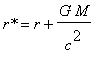
![]() =0,
=0,
![]() . In the vicinity of
. In the vicinity of
![]() V
>>
U
. Then in the vacuum we have
V
>>
U
. Then in the vacuum we have
| > | eq12 := A(x) = x-x[1] + epsilon/2*Int(subs( U(xs)=1/(xs*eta(xs)*A(xs)),xs^2/U(xs) ),xs=x[1]..x); |
![eq12 := A(x) = x-x[1]+1/2*epsilon*Int(`x*`^3*eta(`x*`)*A(`x*`),`x*` = x[1] .. x)](images/rtg_bh80.gif)
| > | eq13 := Diff(A(x),x) = 1 + epsilon/2*x^3*eta(x)*A(x); |
![]()
| > | #let's omit second term in eq8: eq14 := subs( {epsilon=0,xi=0,A=A(x),eta=eta(x)},eq8 ); |
![]()
Let's introduce new function:
| > | #new function: eq15 := f(x) = 1/2*x[1]^3*eta(x)*A(x);#in immediate proximity to x[1] we suppose x = x[1] |
![]()
| > | #from eq13: eq16 := lhs(eq13) = 1 + epsilon*f(x); |
![]()
Hence
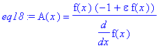
| > | eq17 := eta(x)=solve(eq15,eta(x)); subs(eta(x)=rhs(eq17),eq14): expand( value(%) ); subs(diff(A(x),x)=rhs(eq16),%): eq18 := A(x) = subs(diff(x[1],x)=0,solve(%,A(x)));# NB that we neglected the variation of x^2 in the comparison with eta(x)*A(x) in the vicinity of x[1] |
![eq17 := eta(x) = 2*f(x)/x[1]^3/A(x)](images/rtg_bh85.gif)
![A(x)/f(x)*diff(f(x),x)-3*A(x)/x[1]*diff(x[1],x)-diff(A(x),x)+2 = 0](images/rtg_bh86.gif)
These expressions result in:
| > | eq19 := eta(x) = subs( A(x)=rhs(eq18),rhs(eq17) ); |
![eq19 := eta(x) = 2/x[1]^3/(-1+epsilon*f(x))*diff(f(x),x)](images/rtg_bh88.gif)
Thus we have the expressions for the Riemannian metric:
| > | # U=1/(x*eta*A),V=x/(A*Diff(y,x)^2) eq[8] := U = subs( {eta(x)=rhs(eq19),A(x)=rhs(eq18)},1/(x*eta(x)*A(x)) ); eq[9] := V = subs( A(x)=rhs(eq18),x/(A(x)*Diff(y,x)^2) ); |
![eq[8] := U = 1/2*1/x*x[1]^3/f(x)](images/rtg_bh89.gif)
![eq[9] := V = x/f(x)/(-1+epsilon*f(x))*diff(f(x),x)/Diff(y,x)^2](images/rtg_bh90.gif)
Now we have to find f(x).
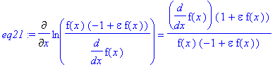
| > | eq20 := subs( A(x)=rhs(eq18),lhs(eq16) ) = rhs(eq16); eq21 := Diff(ln((f(x)*(-1+epsilon*f(x)))/diff(f(x),x)),x) = diff(f(x),x)*(1+epsilon*f(x))/(f(x)*(-1+epsilon*f(x)));# from previous for nonzero diff(f(x),x)/(f(x)*(-1+epsilon*f(x)) |
| > | #verification numer(simplify( value(lhs(eq20)) - rhs(eq20) )): numer(simplify( value(lhs(eq21)) - rhs(eq21) )): %% - %; |
![]()
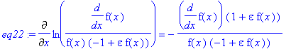
| > | # So, from eq21 eq22 := Diff(ln( diff(f(x),x)/(f(x)*(-1+epsilon*f(x))) ),x) = -rhs(eq21); |
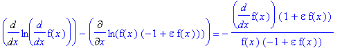
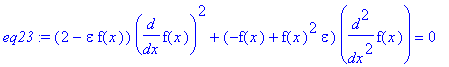
| > | # Hence Diff(ln(diff(f(x),x)),x) - Diff(ln(f(x)*(-1+epsilon*f(x))),x) = rhs(eq22); op(1,lhs(%)) = rhs(%) - value(op(2,lhs(%))): simplify( value(lhs(%)) - rhs(%) = 0 ): eq23 := collect( numer(lhs(%)), {diff(f(x),`$`(x,2)),diff(f(x),x)^2}) = 0; |
But the last expression can be rewritten as:
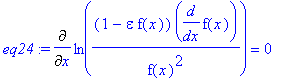
| > | eq24 := Diff(ln((1-epsilon*f(x))*diff(f(x),x)/f(x)^2),x) = 0; #check-up simplify(value(lhs(%))): numer(%): collect(%,{diff(f(x),`$`(x,2)),diff(f(x),x)^2}) - lhs(eq23); |
![]()
Hence
| > | eq25 := (1-epsilon*f(x))*diff(f(x),x)/f(x)^2 = C[0]; |
![eq25 := (1-epsilon*f(x))*diff(f(x),x)/f(x)^2 = C[0]](images/rtg_bh99.gif)
| > | eq[10] := diff(f(x),x) = solve(eq25,diff(f(x),x)); |
![eq[10] := diff(f(x),x) = -C[0]*f(x)^2/(-1+epsilon*f(x))](images/rtg_bh100.gif)
Now the expression for A(x) becomes
| > | ff := subs( diff(f(x),x)=rhs(eq[10]),eq18 ); |
![ff := A(x) = -1/f(x)*(-1+epsilon*f(x))^2/C[0]](images/rtg_bh101.gif)
Since
![]() , the previous equation gives
, the previous equation gives
![f(x[1]) = 1/epsilon](images/rtg_bh103.gif) . Then
. Then
| > | Int(subs( f(x)=`f*`,1/rhs(eq[10]) )*C[0],`f*`=1/epsilon..f) = C[0]*(x-x[1]); value(lhs(%)) = rhs(%): expand(lhs(%)) = rhs(%); |
![Int(-1/`f*`^2*(-1+epsilon*`f*`),`f*` = 1/epsilon .. f) = C[0]*(x-x[1])](images/rtg_bh104.gif)
![]()
| > | eq[11] := -C[0]*(x-x[1]) = epsilon*ln(epsilon*f) + 1/f - epsilon; |
![]()
Next task is a definition of y(x) (outside the matter):
| > | subs( {U=1/(x*eta(x)*A(x)),V=x/(A(x)*Diff(y,x)^2)},fun[3] ): subs(y=y(x),%): simplify( value( % )*(1/x^2/eta(x)*diff(y(x),x)^2)^(1/2) ): eq26 := expand(%*2*x*eta(x)^2); |
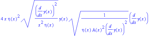
| > | lhs(eq26) - 4*diff(y(x),x)*y(x)*eta(x)/A(x) = 0: eq27 := expand(%/eta(x)); |
| > | Diff(ln(eta(x)),x) = solve(eq14,Diff(ln(eta(x)),x)); |
![]()
| > | op(1,lhs(eq27)) + 2*x*diff(y(x),x)^2/A(x) + op(3,lhs(eq27)) + op(4,lhs(eq27)) = 0: eq28 := expand(A(x)*%/diff(y(x),x)/2); #or eq[12] := A(x)*Diff(x*Diff(y(x),x),x) + x*Diff(y(x),x) - 2*y(x) = 0; |
![]()
Now let's transit from
x
to
f
variable in
![]() .
.
| > | eq29 := lhs(eq[11]/(-C[0])) + x[1] = rhs(eq[11]/(-C[0])) + x[1]; eq30 := Diff(lhs(eq29),f) = diff(rhs(eq29),f); |
![eq29 := x = -1/C[0]*(epsilon*ln(epsilon*f)+1/f-epsilon)+x[1]](images/rtg_bh114.gif)
![eq30 := Diff(x,f) = -1/C[0]*(epsilon/f-1/(f^2))](images/rtg_bh115.gif)
| > | # from eq12, f and previous expression subs(f(x)=f,rhs(ff))*Diff( x(f)*Diff( y(f),f )/rhs(eq30),f)/rhs(eq30) + x(f)*Diff( y(f),f )/rhs(eq30) - 2*y(f): value(%): simplify(%): expand(subs(diff(x(f),f)=rhs(eq30),%)/(-f^3*C[0]*x(f))): eq31 := collect(%,diff(y(f),f)) = 0; |
![eq31 := (1/(f^2*C[0]*x(f))+1/f-1/f/C[0]/x(f)*epsilon)*diff(y(f),f)+2/f^3/C[0]/x(f)*y(f)+diff(y(f),`$`(f,2)) = 0](images/rtg_bh116.gif)
Now let's substitute in eq 31 the next expression:
| > | eq32 := y(f) = x[1]/2 - 1/(C[0]*f)*(1-epsilon*f+epsilon*f*ln(epsilon*f)); |
![eq32 := y(f) = 1/2*x[1]-1/C[0]/f*(1-epsilon*f+epsilon*f*ln(epsilon*f))](images/rtg_bh117.gif)
| > | subs({y(f)=rhs(eq32),x(f)=rhs(eq29)},lhs(eq31)): simplify(%); |
![epsilon/f^2*(ln(epsilon*f)-epsilon*f+1)/(epsilon*f*ln(epsilon*f)+1-epsilon*f-x[1]*C[0]*f)/C[0]](images/rtg_bh118.gif)
| > | # from eq29 the last expression can be rewritten as numer(%)/(-C[0]^2*x*f^3); # which is close to zero in the vicinity of x[1] |
![-epsilon*(ln(epsilon*f)-epsilon*f+1)/C[0]^2/x/f^3](images/rtg_bh119.gif)
| > | # So, from eq32 and eq29 eq[13] := subs(y(f)=y,lhs(eq32) - lhs(eq29) + x) = simplify( rhs(eq32) - rhs(eq29) ) + x; |
![]()
Now U and V can be expressed only through f ( x is the explicit function of f , see eq 29):
| > | eq[14] := subs( f(x)=f,eq[8] ); subs( diff(f(x),x)=rhs(eq[10]),eq[9] ): subs( Diff(y,x)=diff(rhs(eq[13]),x),% ): eq[15] := subs( {diff(x[1],x)=0,f(x)=f},% ); |
![eq[14] := U = 1/2*1/x*x[1]^3/f](images/rtg_bh121.gif)
![eq[15] := V = -x*f/(-1+epsilon*f)^2*C[0]](images/rtg_bh122.gif)
Causality principle
Now we consider the implication of the
causality principle
in our case. Let's
![]() is the unit vector defined by the metric of a spatial section of the Minkowski spacetime:
is the unit vector defined by the metric of a spatial section of the Minkowski spacetime:
![k[i,j]*e^i*e^j = 1](images/rtg_bh124.gif) (
(
![k[i,j] = -mu[i,j]+mu[0,i]*mu[0,k]/mu[0,0]](images/rtg_bh125.gif) , here
i
and
k
are the spatial coordinates). Since
, here
i
and
k
are the spatial coordinates). Since
| > | get_compts(mu)[1,2]; get_compts(mu)[1,3]; get_compts(mu)[1,4]; |
![]()
![]()
![]()
![]() in our case,
in our case,
![k[i,j]*e^i*e^j = 1](images/rtg_bh130.gif) becomes
becomes
| > | -e[1]^2*get_compts(mu)[2,2] - get_compts(mu)[3,3]*e[2]^2 - sin(theta)^2*get_compts(mu)[3,3]*e[3]^2: aa := collect(%,r^2) = 1; |
![]()
Let's introduce the four-velocity vector
 . For isotropic vector
v
=1 (from previous equality). The
causality principle
requires:
. For isotropic vector
v
=1 (from previous equality). The
causality principle
requires:
![g[nu,lambda]*v^nu*v^lambda](images/rtg_bh133.gif) <=
0.
<=
0.
| > | # this is bb := get_compts(g)[1,1] + get_compts(g)[2,2]*e[1]^2 + get_compts(g)[3,3]*e[2]^2 + get_compts(g)[3,3]*e[3]^2*sin(theta)^2: cc := collect(bb,W(r)^2)<=0; |
![]()
| > | solve(aa,e[2]^2+sin(theta)^2*e[3]^2); dd := collect( W(r)^2*(-%) + op(2,lhs(cc)) + op(3,lhs(cc)),e[1]^2 ) <= 0; |
![-(e[1]^2-1)/r^2](images/rtg_bh135.gif)
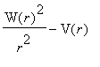
![dd := (W(r)^2/r^2-V(r))*e[1]^2-W(r)^2/r^2+U(r) <= 0](images/rtg_bh136.gif)
If
 >=0 (0<=
![]() <=1) then
<=1) then
![]()
 <=0. Hence
![]() <=
<=
![]() .
.
If
 <=0 (0<=
![]() <=1) then
<=1) then
| > | U(r) - V(r) -(W(r)^2/r^2-V(r))*(1 - e[1]^2) <= 0; simplify(lhs(%) - lhs(dd));# verification |
![U(r)-V(r)-(W(r)^2/r^2-V(r))*(1-e[1]^2) <= 0](images/rtg_bh145.gif)
![]()
Hence again
![]() <=
<=
![]() .
.
From the causality principle we have (since
![f(x[1]) = 1/epsilon](images/rtg_bh149.gif) > 0,
f
is positive within some region of
> 0,
f
is positive within some region of
![]() where
f
changes smoothly):
where
f
changes smoothly):
| > | eq33 := simplify( rhs( eq[14] ) - rhs( eq[15] ) )*2*(-1+epsilon*f)^2*x*f <= 0;# x and f are positive |
![]()
Since
| > | subs({U(r)=rhs(eq[8]),V(r)=rhs(eq[9])}, g_scal )*2/W(r)^4/sin(theta)^2 < 0; |
![-x[1]^3/f(x)^2/(-1+epsilon*f(x))*diff(f(x),x)/Diff(y,x)^2 < 0](images/rtg_bh152.gif)
 and
and
![]() are to have the opposite signs. As a result,
eq
25 suggests the negative sign of
are to have the opposite signs. As a result,
eq
25 suggests the negative sign of
![]() . Then from the positivity of
f
we have for x:
. Then from the positivity of
f
we have for x:
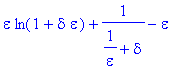
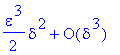
| > | -C[0]*op(1,rhs(eq29)): subs(f=1/epsilon+delta,%):# delta is the small positive quantity expand( simplify(%,ln) ); series(%,delta=0,3); |
Hence
![]() . And from the causality principle we have
. And from the causality principle we have
| > | x >= solve(lhs(subs(x[1]=x1,eq33)) = 0,x)[1]; |
![1/2*1/C[0]*(-2*C[0]*x1)^(1/2)*(-1+epsilon*f)*x1/f <= x](images/rtg_bh159.gif)
Thus,
![]() because an opposite situation would result in the existence of the vacuum region between
because an opposite situation would result in the existence of the vacuum region between
![]() and
and
![]() where the causality principle is violated.
where the causality principle is violated.
Now let's return to the expressions for the Riemannian interval:
| > | eq34 := U = subs( x1=x[1],subs(x=rhs(eq29),subs(x[1]=x1,rhs(eq[14]))) ); eq35 := V = subs(x=rhs(eq29),subs(x[1]=x1,rhs(eq[15]))); |
![eq34 := U = 1/2*1/(-1/C[0]*(epsilon*ln(epsilon*f)+1/f-epsilon)+x[1])*x[1]^3/f](images/rtg_bh163.gif)
![eq35 := V = -(-1/C[0]*(epsilon*ln(epsilon*f)+1/f-epsilon)+x[1])*f/(-1+epsilon*f)^2*C[0]](images/rtg_bh164.gif)
Now we consider the Schwarzschild solution which has to be joined with the obtained one in the limit of
![]() ->0.
->0.
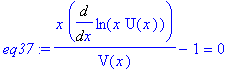
| > | eq36 := subs( {V=V(x),epsilon=0,Diff(y,x)=1},lhs( fun[1] ) ) = 0;# Diff(y,x) from eq13 eq37 := subs( {V=V(x),U=U(x),epsilon=0,Diff(y,x)=1},lhs( fun[2] ) ) = 0; eq38 := dsolve({eq36,eq37},{V(x),U(x)}); |
![]()
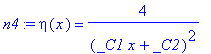
![eq38 := [{V(x) = x/(x+_C2)}, {U(x) = exp(Int((-1+V(x))/x,x))*_C1}]](images/rtg_bh168.gif)
| > | # Hence eq39 := Vs(x) = x/(x+omega); eq40 := Us(x) = simplify( beta*exp(int((-1+x/(x+omega))/x,x)) ); |
![]()
![]()
But
![]() transforms
eq
34 and
eq
35 in:
transforms
eq
34 and
eq
35 in:
| > | subs(epsilon=0,eq29): solve(%,f): subs( f=%,subs( {x[1]=x1,epsilon=0},eq35 ) ): subs(x1=x[1],%); subs(epsilon=0,eq29): solve(%,f): subs( f=%,subs( {x[1]=x1,epsilon=0},eq34 ) ): subs(x1=x[1],%); |
![V = -x/(-x+x[1])](images/rtg_bh172.gif)
![U = 1/2*1/x*x[1]^3*C[0]*(-x+x[1])](images/rtg_bh173.gif)
| > | #Thus eq41 := omega = -x[1]; eq42 := beta = solve( rhs(%%) = subs( omega=-x[1],rhs(eq40) ),beta ); |
![]()
![]()
Since the Schwarzschild metric gives the Minkowski one at infinity, we have
| > | limit(rhs(eq40),x=infinity) = 1; |
![]()
| > | # Hence subs(beta=1,eq42); eq[16] := C[0] = solve(%,C[0]); |
![]()
![eq[16] := C[0] = -2/x[1]^3](images/rtg_bh178.gif)
Thus for the Schwarzschild interval we have:
| > | x=y+1/2; subs( %,subs(x[1]=1,V = x/(x-x[1])) ); subs( %%,subs( x[1]=1,subs( eq[16],U = -1/2*1/x*x[1]^3*C[0]*(x-x[1]) ) ) ); sch[1] := ds^2 = (1-G*M/c^2/r)/(1+GM/c^2/r)*dt^2 - (1+G*M/c^2/r)/(1-GM/c^2/r)*dr^2 - (1+G*M/c^2/r)^2*r^2*(d(theta)^2+sin(theta)^2*d(phi)^2); |
![]()


![sch[1] := ds^2 = (1-G*M/c^2/r)/(1+GM/c^2/r)*dt^2-(1+G*M/c^2/r)/(1-GM/c^2/r)*dr^2-(1+G*M/c^2/r)^2*r^2*(d(theta)^2+sin(theta)^2*d(phi)^2)](images/rtg_bh182.gif)
or in the usual (unshifted) spherical coordinate form (
 ):
):
| > | sch[2] := ds^2 = (1-2*G*M/c^2/`r*`)*dt^2 - 1/(1-2*GM/c^2/`r*`)*d(`r*`)^2 - `r*`^2*(d(theta)^2+sin(theta)^2*d(phi)^2); |
![sch[2] := ds^2 = (1-2*G*M/c^2/`r*`)*dt^2-1/(1-2*GM/c^2/`r*`)*d(`r*`)^2-`r*`^2*(d(theta)^2+sin(theta)^2*d(phi)^2)](images/rtg_bh184.gif)
Thus, we have the following expressions for the Riemannian interval:
| > | eq[17] := collect( simplify( subs( C[0]=rhs(eq[16]),eq29 ) ),x[1] ); eq[18] := collect( simplify( subs( C[0]=rhs(eq[16]),eq34 )),x[1] ); eq[19] := collect( simplify( subs( C[0]=rhs(eq[16]),eq35 ) ),x[1] ); eq[20] := collect( simplify( subs( {x1=x[1],C[0]=rhs(eq[16])},subs(x=rhs(eq29),subs(x[1]=x1,eq[13]) )) ),x[1] ); |
![eq[17] := x = 1/2*(1-epsilon*f+epsilon*f*ln(epsilon*f))/f*x[1]^3+x[1]](images/rtg_bh185.gif)
![eq[18] := U = x[1]^2/((1-epsilon*f+epsilon*f*ln(epsilon*f))*x[1]^2+2*f)](images/rtg_bh186.gif)
![eq[19] := V = (1-epsilon*f+epsilon*f*ln(epsilon*f))/(-1+epsilon*f)^2+2*f/(-1+epsilon*f)^2/x[1]^2](images/rtg_bh187.gif)
![eq[20] := y = 1/2*(1-epsilon*f+epsilon*f*ln(epsilon*f))/f*x[1]^3+1/2*x[1]](images/rtg_bh188.gif)
In contrary to the GR case, U is not 0 at the Schwarzschild sphere due to the massive graviton:
| > | limit(eq[18],f=1/epsilon); limit(eq[19],f=1/epsilon); limit(eq[20],f=1/epsilon); |
![]()
![V = 1/signum(epsilon)^3/signum(x[1])^2*infinity](images/rtg_bh190.gif)
![]()
and the radius of this sphere in the RTG differs from that in the GR:
| > | #from eq11 x[1] = 1 - Int(1/2*epsilon*`x*`^2*(1/U(`x*`)-1/V(`x*`)),`x*` = 0 .. x[1]); # or approximately x[1] = 1 - Int(1/2*epsilon*`x*`^2/U(`x*`),`x*` = 0 .. x[1]); |
![x[1] = 1-Int(1/2*epsilon*`x*`^2*(1/U(`x*`)-1/V(`x*`)),`x*` = 0 .. x[1])](images/rtg_bh192.gif)
![x[1] = 1-Int(1/2*epsilon*`x*`^2/U(`x*`),`x*` = 0 .. x[1])](images/rtg_bh193.gif)
In the vicinity of singularity (i.e.
![]() ) we can expand
f
over the small parameter
) we can expand
f
over the small parameter
 <<1:
<<1:
| > | eq43 := f = 1/epsilon/(1+omega); |
![]()
| > | subs(f=rhs(eq43),eq[17]); eq44 := lhs(%) = series( rhs(%),omega=0,3 ); |
![x = 1/2*(1-1/(1+omega)+1/(1+omega)*ln(1/(1+omega)))*epsilon*(1+omega)*x[1]^3+x[1]](images/rtg_bh197.gif)
![]()
| > | lhs(eq44) - x[1] = convert( rhs(eq44) - x[1],polynom ); eq45 := psi/epsilon = sqrt( lhs(%)/coeff(rhs(%),omega^2) ); eq46 := subs(omega=rhs(eq45),eq43); |
![]()
![eq45 := psi/epsilon = 2*((x-x[1])/epsilon/x[1]^3)^(1/2)](images/rtg_bh200.gif)
![eq46 := f = 1/(epsilon*(1+2*((x-x[1])/epsilon/x[1]^3)^(1/2)))](images/rtg_bh201.gif)
| > | eq[21] := subs( eq46,eq[14] ); eq[22] := simplify( subs( {eq[16],eq46},eq[15] ) ); |
![eq[21] := U = 1/2*1/x*x[1]^3*epsilon*(1+2*((x-x[1])/epsilon/x[1]^3)^(1/2))](images/rtg_bh202.gif)
![eq[22] := V = -1/2*(1+2*(-(-x+x[1])/epsilon/x[1]^3)^(1/2))*x/(-x+x[1])](images/rtg_bh203.gif)
Hence for
eq45
<<1 and in the vicinity of
![]() =1:
=1:
| > | lhs(eq[21]) = subs( {x=1,epsilon=(1/2)*(2*G*M*m/(c*`h*`))^2},subs( x[1]=1,op( 1,rhs(expand(eq[21])) ) ) );# `h*`=h/2/Pi is the Dirac's constant subs(x[1]=1,eq[13]): eq47 := x = solve(%,x); lhs(eq[22]) = subs( %,subs( x[1]=1,op( 1,rhs(expand(eq[22])) ) ) ); |
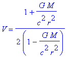
![]()
| > | # Hence V = 1/2*(1+G*M/c^2/r^2)/(1-G*M/c^2/r^2); |
| > | # and in the vicinity of the Schwarzschild sphere the corrected interval is logunov := ds^2 = G^2*M^2*m^2/c^2/`h*`^2*dt^2 - 1/(1-2*GM/c^2/`r*`)/2*d(`r*`)^2 - `r*`^2*(d(theta)^2+sin(theta)^2*d(phi)^2); |
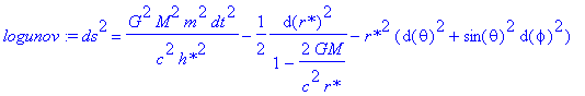
Now we shall made some numerical estimations for the above considered metric. For the upper estimation of the graviton mass we choose
m
=
 g [
S.S.Gerstein, A.A.Logunov, M.A.Mestvirishvili, arXiv:astro-ph/0302412] (however, compare this Ref. with
V.L.Kalashnikov, arXiv:gr-qc/0208070) and shall consider the source with the mass which is equal to 10
g [
S.S.Gerstein, A.A.Logunov, M.A.Mestvirishvili, arXiv:astro-ph/0302412] (however, compare this Ref. with
V.L.Kalashnikov, arXiv:gr-qc/0208070) and shall consider the source with the mass which is equal to 10
![]() .
.
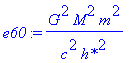
| > | n1 := epsilon = subs( {G=6.67e-8,c=3e10,hh=1.054e-27,M=10*2e33,m=1.6e-66},(1/2)*(2*G*M*m/hh/c)^2 ); |
![]()
Now we return to the above obtained equations:
| > | n2 := eq14; n3 := diff(A(x),x) = 1 + epsilon*x^2*A(x)/2*(x*eta(x) - 1/x);# taking into account eq10 and supposing diff(y,x)=1 |
![]()
![]()
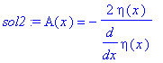
| > | sol1 := dsolve({n2,n3},{A(x),eta(x)}); |
![sol1 := [{diff(eta(x),`$`(x,2)) = 1/2*(3*diff(eta(x),x)^2-diff(eta(x),x)*epsilon*x^3*eta(x)^2+eta(x)*diff(eta(x),x)*epsilon*x)/eta(x)}, {A(x) = -2*eta(x)/diff(eta(x),x)}]](images/rtg_bh215.gif)
Thus
| > | sol2 := A(x) = -2*eta(x)/diff(eta(x),x); ODE := diff(eta(x),`$`(x,2)) = 1/2*(3*diff(eta(x),x)^2-diff(eta(x),x)*epsilon*x^3*eta(x)^2+eta(x)*diff(eta(x),x)*epsilon*x)/eta(x); |
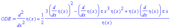
The latter equation requires a numerical consideration. Let's define the initial data from the solution for the Schwarzschild metric. For zero graviton mass we have:
| > | # GR case (epsilon=0) subs( epsilon=0,ODE ); n4 := dsolve(%,eta(x)); n5 := value( subs(%,sol2 ) ); |
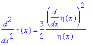
![]()
or returning to the old variables:
| > | U = subs( {n4,n5},1/(x*eta(x)*A(x)) ); V = subs( n5,x/A(x) ); |
![]()
![]()
| > | # Hence solve( {1/4/x*(_C1*x+_C2)*_C1 = (x-1)/x,x/(_C1*x+_C2)*_C1 = x/(x-1)}, {_C1,_C2}); |
![]()
In the vicinity of the Schwarzschild singularity the high numerical accuracy is required. We define the initial and final points and shall perform the simulation in the logarithmic scale.
| > | Digits := 200: Digits; begin := evalf(1.+1e-42);# initial x et := subs(x=begin,1/(x-1)^2);# initial eta from Schwarzschild metric d_et := subs( x=begin,diff(1/(x-1)^2,x) );# its derivative |
![]()
![]()
![]()
![]()
| > | en1 := evalf(1. + 10^(-43.69)): en2 := evalf(1. + 10^(-45)): |
| > | ic1 := eta(begin) = et, D(eta)(begin) = d_et: dsol1 := dsolve( {subs(epsilon=rhs(n1),ODE),ic1}, type=numeric, startinit=false, range = begin..en1, output=procedurelist ); dsol2 := dsolve( {subs(epsilon=0,ODE),ic1}, type=numeric, startinit=false, range = begin..en2, output=procedurelist ); |
![]()
![]()
| > | i := 'i': sol_deta1 := array(1..1000): sol_eta1 := array(1..1000): sol_x1 := array(1..1000): for i from 1 to 1000 do z := evalf(1. + 10^(-42.-1.69*i/1000)): sol_deta1[i] := rhs(dsol1(z)[3]): sol_eta1[i] := rhs(dsol1(z)[2]): sol_x1[i] := rhs(dsol1(z)[1]): od: i := 'i': sol_deta2 := array(1..1000): sol_eta2 := array(1..1000): sol_x2 := array(1..1000): for i from 1 to 1000 do z := evalf(1. + 10^(-42.-3.*i/1000)): sol_deta2[i] := rhs(dsol2(z)[3]): sol_eta2[i] := rhs(dsol2(z)[2]): sol_x2[i] := rhs(dsol2(z)[1]): od: |
The resulting behavior of the metric in the vicinity of the Schwarzschild singularity has the following form (red and green curves correspond to the Schwarzschild's and Logunov's metrics, respectively; point is the result of the analytical estimation).
| > | s1 := [log10( evalf(1. + 10^(-43.69)) - 1. )]: s2 := [log10( rhs(n1)/2. )]: g1 := statplots[scatterplot](s1, s2, symbolsize=15, color = black): plot([[log10(sol_x1[k]-1.),log10( 1./(sol_eta1[k]*sol_x1[k]*(-2.*sol_eta1[k]/sol_deta1[k])) )] $k=1..1000],color=green,axes=boxed): plot([[log10(sol_x2[k]-1.),log10( 1./(sol_eta2[k]*sol_x2[k]*(-2.*sol_eta2[k]/sol_deta2[k])) )] $k=1..1000],color=red,axes=boxed): display(%,%%,g1,view=[-42..-45,-42..-45], title=`log(U) vs. log(x-1)`); plot([[log10(sol_x1[k]-1.),log10( sol_x1[k]/(-2.*sol_eta1[k]/sol_deta1[k]) )] $k=1..1000],color=green,axes=boxed): plot([[log10(sol_x2[k]-1.),log10( sol_x2[k]/(-2.*sol_eta2[k]/sol_deta2[k]) )] $k=1..1000],color=red,axes=boxed): display(%,%%,view=[-42..-45,42..45.5], title=`log(V) vs. log(x-1)`); |
![[Maple Plot]](images/rtg_bh230.gif)
![[Maple Plot]](images/rtg_bh231.gif)
We can see that
![]() ,
,
![limit(V,x = x[1])](images/rtg_bh233.gif) =
=
![]() ,
,
![limit(U,x = x[1])](images/rtg_bh235.gif) =
=
![]() . The interval where the corrected metric differs from the Schwarzschild solution is extremely small (~
. The interval where the corrected metric differs from the Schwarzschild solution is extremely small (~
![]() ). As a result, the correct investigation of the singularity vicinity requires taking into account the quantum effects.
). As a result, the correct investigation of the singularity vicinity requires taking into account the quantum effects.
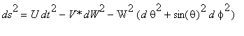
Spherically symmetric collapse
In the beginning let us consider the radially falling particle in the framework of the RTG. The motion is described by the geodesic line equations in the effective Rimannian spacetime::
| > | eqns:= geodesic_eqns( coord, s, Cf2 ); |
| > | eqns[4]; |
Since
 , we have
 =
=
 and
and
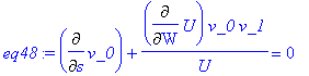
| > | eq48 := Diff(v_0,s) + 1/U*Diff(U,W)*v_0*v_1 = 0;# v_0=diff(t,s), v_1=diff(W,s) |
Hence
| > | eq49 := Diff(ln(v_0*U),s) = 0; |
![]()
Thus
| > | eq50 := v_0 = U0/U;# U0 is some constant |
![]()
It is convenient to transit from
r
to
W
in interval
 that gives
 . Since for the four-velocity
![g[k,l]*v^k*v^l = 1](images/rtg_bh251.gif) , we have
, we have
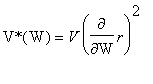
| > | macro(Vs=`V*`): eq51 := U*rhs(eq50)^2 - Vs*Diff(W,s)^2 = 1; |
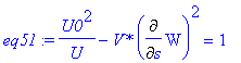
If an initial velocity equals zero, then
| > | subs( {U0=1,W=W(s)},eq51 ): solve(%,Diff(W(s),s)); |
![]()
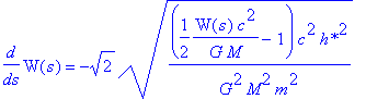
| > | eq52 := diff(W(s),s) = -sqrt((1-U)/(U*Vs)); |
![]()
| > | # Since diff(subs( x[1]=x1,rhs(eq[13]) ),x); # we have Vs = subs(eq[16],rhs(eq[15])); eq[14]; simplify( lhs(eq52) = -sqrt(1-U)/sqrt(rhs(%)*rhs(%%)) ); |
![]()
![`V*` = 2*x*f/(-1+epsilon*f)^2/x[1]^3](images/rtg_bh256.gif)
![U = 1/2*1/x*x[1]^3/f](images/rtg_bh257.gif)
![]()
| > | # That is eq53 := diff(W(s),s) = -(1-U)^(1/2)*(1-epsilon*f); |
![]()
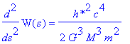
Hence in the vicinity of
![]() we have (
U
is close to zero, see above):
we have (
U
is close to zero, see above):
| > | lhs(subs({eq43,U=0},eq53)) = convert( series( rhs(subs({eq43,U=0},eq53)),omega=0,2 ),polynom): eq54 := subs(omega=rhs(eq45),%); |
![eq54 := diff(W(s),s) = -2*((x-x[1])/epsilon/x[1]^3)^(1/2)](images/rtg_bh261.gif)
or returning to the dimensional values:
| > | subs( x[1]=1,eq54 ): subs( {epsilon=(1/2)*(2*G*M*m/(c*`h*`))^2,x=W(s)/(2*G*M/c^2)},% ); # or eq[23] := lhs(%) = -(`h*`*c^2)/(G*M*m)*sqrt(W(s)/(G*M)*(1 - 2*G*M/(c^2*W(s)))); |
![eq[23] := diff(W(s),s) = -`h*`*c^2/G/M/m*(W(s)/G/M*(1-2*G*M/c^2/W(s)))^(1/2)](images/rtg_bh263.gif)
Thus, in the vicinity of the Schwarzschild sphere there exists the turning point providing the strong repulsing acceleration:
| > | simplify( diff(eq[23],s) ): lhs(%) = simplify( subs(eq[23],rhs(%)) ); |
Now let's make some numerical estimations of the above obtained results (eq52, and expressions of U and V through A and
![]() ).
).
| > | begin := evalf(1.+1e-42);# initial x et := subs(x=begin,1/(x-1)^2);# initial eta from Schwarzschild metric d_et := subs( x=begin,diff(1/(x-1)^2,x) );# its derivative en1 := evalf(1. + 10^(-43.69)): en2 := evalf(1. + 10^(-45)): ic1 := eta(begin) = et, D(eta)(begin) = d_et: dsol1 := dsolve( {subs(epsilon=rhs(n1),ODE),ic1}, type=numeric, startinit=false, range = begin..en1, output=procedurelist ); dsol2 := dsolve( {subs(epsilon=0,ODE),ic1}, type=numeric, startinit=false, range = begin..en2, output=procedurelist ); i := 'i': sol_deta1 := array(1..1000): sol_eta1 := array(1..1000): sol_x1 := array(1..1000): for i from 1 to 1000 do z := evalf(1. + 10^(-42.-1.69*i/1000)): sol_deta1[i] := rhs(dsol1(z)[3]): sol_eta1[i] := rhs(dsol1(z)[2]): sol_x1[i] := rhs(dsol1(z)[1]): od: i := 'i': sol_deta2 := array(1..1000): sol_eta2 := array(1..1000): sol_x2 := array(1..1000): for i from 1 to 1000 do z := evalf(1. + 10^(-42.-3.*i/1000)): sol_deta2[i] := rhs(dsol2(z)[3]): sol_eta2[i] := rhs(dsol2(z)[2]): sol_x2[i] := rhs(dsol2(z)[1]): od: |
![]()
![]()
![]()
![]()
![]()
| > | -sqrt( 4.*sol_eta1[j]^3/sol_deta1[j]^2 - 1./(sol_x1[j]/(-2.*sol_eta1[j]/sol_deta1[j]))): p1 := plot([[log10(sol_x1[j]-1.),%] $j=1..1000],color=green,axes=boxed): -sqrt( 4.*sol_eta2[j]^3/sol_deta2[j]^2 - 1../(sol_x2[j]/(-2.*sol_eta2[j]/sol_deta2[j]))): p2 := plot([[log10(sol_x2[j]-1.),%] $j=1..1000],color=red,axes=boxed): display(p1,p2); |
![[Maple Plot]](images/rtg_bh271.gif)
| > | display(%,view=[-44..-36,-1..0]); |
![[Maple Plot]](images/rtg_bh272.gif)
Stability analysis
To consider the stability of the analytically obtained metric (expression named as " logunov ", see above) we shall confine oneself to the linear perturbation analysis (S. Chandrasekhar, " The mathematical theory of black holes ", Clarendon Press, 1983, Ch. 4). Let's write the perturbed metric in the following form:
| > | coord := [t, r, theta, phi]:# spherical coordinates gp_compts := array(symmetric,sparse,1..4,1..4): gp_compts[1,1] := U(r):#dt^2 gp_compts[1,4] := W(r)^2*sin(theta)^2*delta*omega(t,r,theta):#dt*dphi gp_compts[2,2] := -V(r):#dr^2 gp_compts[3,3] := -W(r)^2:#dtheta^2 gp_compts[3,4] := W(r)^2*sin(theta)^2*delta*q3(t,r,theta):#dtheta*dphi gp_compts[4,4] := -W(r)^2*sin(theta)^2:#dphi^2 gp_compts[4,2] := W(r)^2*sin(theta)^2*delta*q2(t,r,theta):#dphi*dr gp_compts[4,3] := W(r)^2*sin(theta)^2*delta*q3(t,r,theta):#dphi*dtheta gp := create([-1,-1], eval(gp_compts));# covariant components of metric gpinv := invert( gp, 'detg' ):# contravariant components of metric gp_scal := det(get_compts(gp)):# scalar of the metric tensor |
![]()
![gp := TABLE([index_char = [-1, -1], compts = matrix([[U(r), 0, 0, W(r)^2*sin(theta)^2*delta*omega(t,r,theta)], [0, -V(r), 0, W(r)^2*sin(theta)^2*delta*q2(t,r,theta)], [0, 0, -W(r)^2, W(r)^2*sin(theta)^...](images/rtg_bh274.gif)
![]()
Here
![]() ,
,
![]() and
and
![]() are the perturbation functions,
are the perturbation functions,
![]() is the small perturbation parameter. In the framework of the linear analysis we have to keep only terms which are linear in respect to
is the small perturbation parameter. In the framework of the linear analysis we have to keep only terms which are linear in respect to
![]() . Then perturbed
. Then perturbed
![]() -tensor is:
-tensor is:
| > | ggp_compts := array(symmetric,sparse,1..4,1..4): ggp_compts[1,1] := subs( delta^2=0,simplify( sqrt( -gp_scal )*get_compts(gpinv)[1,1],symbolic,radical ) ):#dt^2 ggp_compts[1,4] := subs( delta^2=0,simplify( sqrt( -gp_scal )*get_compts(gpinv)[1,4],symbolic,radical ) ):#dt*dr ggp_compts[2,2] := subs( delta^2=0,simplify( sqrt( -gp_scal )*get_compts(gpinv)[2,2],symbolic,radical ) ):#dr^2 ggp_compts[3,3] := subs( delta^2=0,simplify( sqrt( -gp_scal )*get_compts(gpinv)[3,3],symbolic,radical ) ):#dtheta^2 ggp_compts[3,4] := subs( delta^2=0,simplify( sqrt( -gp_scal )*get_compts(gpinv)[3,4],symbolic,radical ) ):#dtheta*dphi ggp_compts[4,4] := subs( delta^2=0,simplify( sqrt( -gp_scal )*get_compts(gpinv)[4,4],symbolic,radical ) ):#dphi^2 ggp_compts[4,2] := subs( delta^2=0,simplify( sqrt( -gp_scal )*get_compts(gpinv)[4,2],symbolic,radical ) ):#dphi*dr ggp_compts[4,3] := subs( delta^2=0,simplify( sqrt( -gp_scal )*get_compts(gpinv)[4,3],symbolic,radical ) ):#dtheta*dphi `gp*` := create([1,1], eval(ggp_compts)); |
![]()
![]()
![`gp*` := TABLE([index_char = [1, 1], compts = matrix([[(U(r)*V(r)*W(r)^4*sin(theta)^2)^(1/2)/U(r), 0, 0, (U(r)*V(r)*W(r)^4*sin(theta)^2)^(1/2)*delta*omega(t,r,theta)/U(r)], [0, -(U(r)*V(r)*W(r)^4*sin(t...](images/rtg_bh284.gif)
![`gp*` := TABLE([index_char = [1, 1], compts = matrix([[(U(r)*V(r)*W(r)^4*sin(theta)^2)^(1/2)/U(r), 0, 0, (U(r)*V(r)*W(r)^4*sin(theta)^2)^(1/2)*delta*omega(t,r,theta)/U(r)], [0, -(U(r)*V(r)*W(r)^4*sin(t...](images/rtg_bh285.gif)
![`gp*` := TABLE([index_char = [1, 1], compts = matrix([[(U(r)*V(r)*W(r)^4*sin(theta)^2)^(1/2)/U(r), 0, 0, (U(r)*V(r)*W(r)^4*sin(theta)^2)^(1/2)*delta*omega(t,r,theta)/U(r)], [0, -(U(r)*V(r)*W(r)^4*sin(t...](images/rtg_bh286.gif)
![`gp*` := TABLE([index_char = [1, 1], compts = matrix([[(U(r)*V(r)*W(r)^4*sin(theta)^2)^(1/2)/U(r), 0, 0, (U(r)*V(r)*W(r)^4*sin(theta)^2)^(1/2)*delta*omega(t,r,theta)/U(r)], [0, -(U(r)*V(r)*W(r)^4*sin(t...](images/rtg_bh287.gif)
![`gp*` := TABLE([index_char = [1, 1], compts = matrix([[(U(r)*V(r)*W(r)^4*sin(theta)^2)^(1/2)/U(r), 0, 0, (U(r)*V(r)*W(r)^4*sin(theta)^2)^(1/2)*delta*omega(t,r,theta)/U(r)], [0, -(U(r)*V(r)*W(r)^4*sin(t...](images/rtg_bh288.gif)
![]()
Its covariant derivative on the background metric is:
| > | # the covariant derivative on the background metric A1 := partial_diff( `gp*`, coord ): A2 := contract(A1,[2,3]): d1mu:= d1metric(mu, coord): Cf1:= Christoffel1 ( d1mu ): Cf2:= Christoffel2 ( muinv, Cf1 ): ZZZ := prod(Cf2,`gp*`): A3 := contract(ZZZ,[2,5] ): A4 := contract(A3,[2,3]): simplify(get_compts(A2)[1] + get_compts(A4)[1]); e55 := simplify(get_compts(A2)[2] + get_compts(A4)[2]); simplify(get_compts(A2)[3] + get_compts(A4)[3]); e56 := simplify(get_compts(A2)[4] + get_compts(A4)[4]); |
![]()
![]()
![]()
![]()
![]()
![]()
![]()
![]()
![]()
![]()
![]()
![]()
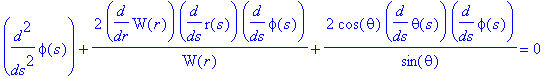
We don't consider first unperturbed equation. The second equation results in:
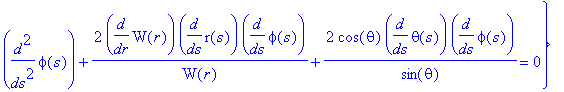
| > | factor( numer( e56 ) ): expand( %/(W(r)^2*(cos(theta)-1)*(cos(theta)+1))/delta ): e58 := factor(%); |
![]()
![]()
![]()
and taking into account the metric coefficients from logunov :
| > | value( subs( {U(r)=epsilon/2,V(r)=1/2/(1-rg/r),W(r)=r},e58 ) ): simplify(%): numer(%): eq[23] := expand(%/r^3/sin(theta)); |
![]()
![]()
In the framework of the linear analysis the time-dependence can be written in the simple harmonic form:
| > | f1 := q2(t,r,theta) = q2(r,theta)*exp(I*sigma*t); f2 := q3(t,r,theta) = q3(r,theta)*exp(I*sigma*t); f3 := omega(t,r,theta) = omega(r,theta)*exp(I*sigma*t); |
![]()
![]()
![]()
Hence
| > | value( subs( {f1,f2,f3},eq[23] ) ): expand( %/exp(sigma*t*I) ); |
![]()
It is obviously that
![]() can not depend on
t
and we can suppose:
can not depend on
t
and we can suppose:
| > | f4 := omega(t,r,theta) = 0; |
![]()
and there is some constraint on the perturbation functions:
| > | value( subs( {f1,f2,f4},eq[23] ) ): eq[24] := expand( %/exp(sigma*t*I)/epsilon ) = 0; |
![]()
Now let us consider the Logunov's field equations for the linearly perturbed spherically symmetric collapsar:
| > | # construction of the Einstein's tensor D1gp := d1metric ( gp, coord ): D2gp := d2metric ( D1gp, coord ): Cf1p := Christoffel1 ( D1gp ): RMN := Riemann( gpinv, D2gp, Cf1p ): RICCI := Ricci( gpinv, RMN ):# Ricci tensor RS := Ricciscalar( gpinv, RICCI ):# Ricci scalar Estnp := raise(gpinv, Einstein( gp, RICCI, RS ), 2 ):# Einstein's tensor with mixed indexes # massive term in the Logunov's equations Z := prod(gpinv,mu): term2 := contract(Z,[2,3]):# second term in brackets (field equation) ZZ := contract(Z,[2,4]): prod(K,contract(ZZ,[1,2])): term3 := prod(table([index_char = [], compts = -1/2]),%):# third term in brackets Lgvp_compts := array(symmetric,sparse,1..4,1..4): Lgvp_compts[1,1] := simplify( subs( {delta^2=0,delta^4=0},get_compts(Estnp)[1,1] - ( epsilon )*( get_compts(K)[1,1] + get_compts(term2)[1,1] + get_compts(term3)[1,1] ) ) ): Lgvp_compts[1,2] := simplify( subs( {delta^2=0,delta^4=0},get_compts(Estnp)[1,2] - ( epsilon )*( get_compts(K)[1,2] + get_compts(term2)[1,2] + get_compts(term3)[1,2] ) ) ): Lgvp_compts[1,3] := simplify( subs( {delta^2=0,delta^4=0},get_compts(Estnp)[1,3] - ( epsilon )*( get_compts(K)[1,3] + get_compts(term2)[1,3] + get_compts(term3)[1,3] ) ) ): Lgvp_compts[1,4] := simplify( subs( {delta^2=0,delta^4=0},get_compts(Estnp)[1,4] - ( epsilon )*( get_compts(K)[1,4] + get_compts(term2)[1,4] + get_compts(term3)[1,4] ) ) ): Lgvp_compts[2,2] := simplify( subs( {delta^2=0,delta^4=0},get_compts(Estnp)[2,2] - ( epsilon )*( get_compts(K)[2,2] + get_compts(term2)[2,2] + get_compts(term3)[2,2] ) ) ): Lgvp_compts[2,3] := simplify( subs( {delta^2=0,delta^4=0},get_compts(Estnp)[2,3] - ( epsilon )*( get_compts(K)[2,3] + get_compts(term2)[2,3] + get_compts(term3)[2,3] ) ) ): Lgvp_compts[2,4] := simplify( subs( {delta^2=0,delta^4=0},get_compts(Estnp)[2,4] - ( epsilon )*( get_compts(K)[2,4] + get_compts(term2)[2,4] + get_compts(term3)[2,4] ) ) ): Lgvp_compts[3,3] := simplify( subs( {delta^2=0,delta^4=0},get_compts(Estnp)[3,3] - ( epsilon )*( get_compts(K)[3,3] + get_compts(term2)[3,3] + get_compts(term3)[3,3] ) ) ): Lgvp_compts[3,4] := simplify( subs( {delta^2=0,delta^4=0},get_compts(Estnp)[3,4] - ( epsilon )*( get_compts(K)[3,4] + get_compts(term2)[3,4] + get_compts(term3)[3,4] ) ) ): Lgvp_compts[4,4] := simplify( subs( {delta^2=0,delta^4=0},get_compts(Estnp)[4,4] - ( epsilon )*( get_compts(K)[4,4] + get_compts(term2)[4,4] + get_compts(term3)[4,4] ) ) ): Lgvp := act(expand,create([-1,1], eval(Lgvp_compts)));# left-hand side of "massive" field equation |
![]()
![]()
![Lgvp := TABLE([index_char = [-1, 1], compts = matrix([[-1/(W(r)^2)+2/W(r)/V(r)*diff(W(r),`$`(r,2))-1/W(r)/V(r)^2*diff(V(r),r)*diff(W(r),r)+1/W(r)^2/V(r)*diff(W(r),r)^2-epsilon-1/2*1/U(r)*epsilon+1/2*1/...](images/rtg_bh316.gif)
![Lgvp := TABLE([index_char = [-1, 1], compts = matrix([[-1/(W(r)^2)+2/W(r)/V(r)*diff(W(r),`$`(r,2))-1/W(r)/V(r)^2*diff(V(r),r)*diff(W(r),r)+1/W(r)^2/V(r)*diff(W(r),r)^2-epsilon-1/2*1/U(r)*epsilon+1/2*1/...](images/rtg_bh317.gif)
![Lgvp := TABLE([index_char = [-1, 1], compts = matrix([[-1/(W(r)^2)+2/W(r)/V(r)*diff(W(r),`$`(r,2))-1/W(r)/V(r)^2*diff(V(r),r)*diff(W(r),r)+1/W(r)^2/V(r)*diff(W(r),r)^2-epsilon-1/2*1/U(r)*epsilon+1/2*1/...](images/rtg_bh318.gif)
![Lgvp := TABLE([index_char = [-1, 1], compts = matrix([[-1/(W(r)^2)+2/W(r)/V(r)*diff(W(r),`$`(r,2))-1/W(r)/V(r)^2*diff(V(r),r)*diff(W(r),r)+1/W(r)^2/V(r)*diff(W(r),r)^2-epsilon-1/2*1/U(r)*epsilon+1/2*1/...](images/rtg_bh319.gif)
![Lgvp := TABLE([index_char = [-1, 1], compts = matrix([[-1/(W(r)^2)+2/W(r)/V(r)*diff(W(r),`$`(r,2))-1/W(r)/V(r)^2*diff(V(r),r)*diff(W(r),r)+1/W(r)^2/V(r)*diff(W(r),r)^2-epsilon-1/2*1/U(r)*epsilon+1/2*1/...](images/rtg_bh320.gif)
![Lgvp := TABLE([index_char = [-1, 1], compts = matrix([[-1/(W(r)^2)+2/W(r)/V(r)*diff(W(r),`$`(r,2))-1/W(r)/V(r)^2*diff(V(r),r)*diff(W(r),r)+1/W(r)^2/V(r)*diff(W(r),r)^2-epsilon-1/2*1/U(r)*epsilon+1/2*1/...](images/rtg_bh321.gif)
![Lgvp := TABLE([index_char = [-1, 1], compts = matrix([[-1/(W(r)^2)+2/W(r)/V(r)*diff(W(r),`$`(r,2))-1/W(r)/V(r)^2*diff(V(r),r)*diff(W(r),r)+1/W(r)^2/V(r)*diff(W(r),r)^2-epsilon-1/2*1/U(r)*epsilon+1/2*1/...](images/rtg_bh322.gif)
![Lgvp := TABLE([index_char = [-1, 1], compts = matrix([[-1/(W(r)^2)+2/W(r)/V(r)*diff(W(r),`$`(r,2))-1/W(r)/V(r)^2*diff(V(r),r)*diff(W(r),r)+1/W(r)^2/V(r)*diff(W(r),r)^2-epsilon-1/2*1/U(r)*epsilon+1/2*1/...](images/rtg_bh323.gif)
![Lgvp := TABLE([index_char = [-1, 1], compts = matrix([[-1/(W(r)^2)+2/W(r)/V(r)*diff(W(r),`$`(r,2))-1/W(r)/V(r)^2*diff(V(r),r)*diff(W(r),r)+1/W(r)^2/V(r)*diff(W(r),r)^2-epsilon-1/2*1/U(r)*epsilon+1/2*1/...](images/rtg_bh324.gif)
![Lgvp := TABLE([index_char = [-1, 1], compts = matrix([[-1/(W(r)^2)+2/W(r)/V(r)*diff(W(r),`$`(r,2))-1/W(r)/V(r)^2*diff(V(r),r)*diff(W(r),r)+1/W(r)^2/V(r)*diff(W(r),r)^2-epsilon-1/2*1/U(r)*epsilon+1/2*1/...](images/rtg_bh325.gif)
![Lgvp := TABLE([index_char = [-1, 1], compts = matrix([[-1/(W(r)^2)+2/W(r)/V(r)*diff(W(r),`$`(r,2))-1/W(r)/V(r)^2*diff(V(r),r)*diff(W(r),r)+1/W(r)^2/V(r)*diff(W(r),r)^2-epsilon-1/2*1/U(r)*epsilon+1/2*1/...](images/rtg_bh326.gif)
![Lgvp := TABLE([index_char = [-1, 1], compts = matrix([[-1/(W(r)^2)+2/W(r)/V(r)*diff(W(r),`$`(r,2))-1/W(r)/V(r)^2*diff(V(r),r)*diff(W(r),r)+1/W(r)^2/V(r)*diff(W(r),r)^2-epsilon-1/2*1/U(r)*epsilon+1/2*1/...](images/rtg_bh327.gif)
![Lgvp := TABLE([index_char = [-1, 1], compts = matrix([[-1/(W(r)^2)+2/W(r)/V(r)*diff(W(r),`$`(r,2))-1/W(r)/V(r)^2*diff(V(r),r)*diff(W(r),r)+1/W(r)^2/V(r)*diff(W(r),r)^2-epsilon-1/2*1/U(r)*epsilon+1/2*1/...](images/rtg_bh328.gif)
![Lgvp := TABLE([index_char = [-1, 1], compts = matrix([[-1/(W(r)^2)+2/W(r)/V(r)*diff(W(r),`$`(r,2))-1/W(r)/V(r)^2*diff(V(r),r)*diff(W(r),r)+1/W(r)^2/V(r)*diff(W(r),r)^2-epsilon-1/2*1/U(r)*epsilon+1/2*1/...](images/rtg_bh329.gif)
![Lgvp := TABLE([index_char = [-1, 1], compts = matrix([[-1/(W(r)^2)+2/W(r)/V(r)*diff(W(r),`$`(r,2))-1/W(r)/V(r)^2*diff(V(r),r)*diff(W(r),r)+1/W(r)^2/V(r)*diff(W(r),r)^2-epsilon-1/2*1/U(r)*epsilon+1/2*1/...](images/rtg_bh330.gif)
![Lgvp := TABLE([index_char = [-1, 1], compts = matrix([[-1/(W(r)^2)+2/W(r)/V(r)*diff(W(r),`$`(r,2))-1/W(r)/V(r)^2*diff(V(r),r)*diff(W(r),r)+1/W(r)^2/V(r)*diff(W(r),r)^2-epsilon-1/2*1/U(r)*epsilon+1/2*1/...](images/rtg_bh331.gif)
![Lgvp := TABLE([index_char = [-1, 1], compts = matrix([[-1/(W(r)^2)+2/W(r)/V(r)*diff(W(r),`$`(r,2))-1/W(r)/V(r)^2*diff(V(r),r)*diff(W(r),r)+1/W(r)^2/V(r)*diff(W(r),r)^2-epsilon-1/2*1/U(r)*epsilon+1/2*1/...](images/rtg_bh332.gif)
![Lgvp := TABLE([index_char = [-1, 1], compts = matrix([[-1/(W(r)^2)+2/W(r)/V(r)*diff(W(r),`$`(r,2))-1/W(r)/V(r)^2*diff(V(r),r)*diff(W(r),r)+1/W(r)^2/V(r)*diff(W(r),r)^2-epsilon-1/2*1/U(r)*epsilon+1/2*1/...](images/rtg_bh333.gif)
![Lgvp := TABLE([index_char = [-1, 1], compts = matrix([[-1/(W(r)^2)+2/W(r)/V(r)*diff(W(r),`$`(r,2))-1/W(r)/V(r)^2*diff(V(r),r)*diff(W(r),r)+1/W(r)^2/V(r)*diff(W(r),r)^2-epsilon-1/2*1/U(r)*epsilon+1/2*1/...](images/rtg_bh334.gif)
![Lgvp := TABLE([index_char = [-1, 1], compts = matrix([[-1/(W(r)^2)+2/W(r)/V(r)*diff(W(r),`$`(r,2))-1/W(r)/V(r)^2*diff(V(r),r)*diff(W(r),r)+1/W(r)^2/V(r)*diff(W(r),r)^2-epsilon-1/2*1/U(r)*epsilon+1/2*1/...](images/rtg_bh335.gif)
![Lgvp := TABLE([index_char = [-1, 1], compts = matrix([[-1/(W(r)^2)+2/W(r)/V(r)*diff(W(r),`$`(r,2))-1/W(r)/V(r)^2*diff(V(r),r)*diff(W(r),r)+1/W(r)^2/V(r)*diff(W(r),r)^2-epsilon-1/2*1/U(r)*epsilon+1/2*1/...](images/rtg_bh336.gif)
![Lgvp := TABLE([index_char = [-1, 1], compts = matrix([[-1/(W(r)^2)+2/W(r)/V(r)*diff(W(r),`$`(r,2))-1/W(r)/V(r)^2*diff(V(r),r)*diff(W(r),r)+1/W(r)^2/V(r)*diff(W(r),r)^2-epsilon-1/2*1/U(r)*epsilon+1/2*1/...](images/rtg_bh337.gif)
![Lgvp := TABLE([index_char = [-1, 1], compts = matrix([[-1/(W(r)^2)+2/W(r)/V(r)*diff(W(r),`$`(r,2))-1/W(r)/V(r)^2*diff(V(r),r)*diff(W(r),r)+1/W(r)^2/V(r)*diff(W(r),r)^2-epsilon-1/2*1/U(r)*epsilon+1/2*1/...](images/rtg_bh338.gif)
![Lgvp := TABLE([index_char = [-1, 1], compts = matrix([[-1/(W(r)^2)+2/W(r)/V(r)*diff(W(r),`$`(r,2))-1/W(r)/V(r)^2*diff(V(r),r)*diff(W(r),r)+1/W(r)^2/V(r)*diff(W(r),r)^2-epsilon-1/2*1/U(r)*epsilon+1/2*1/...](images/rtg_bh339.gif)
![Lgvp := TABLE([index_char = [-1, 1], compts = matrix([[-1/(W(r)^2)+2/W(r)/V(r)*diff(W(r),`$`(r,2))-1/W(r)/V(r)^2*diff(V(r),r)*diff(W(r),r)+1/W(r)^2/V(r)*diff(W(r),r)^2-epsilon-1/2*1/U(r)*epsilon+1/2*1/...](images/rtg_bh340.gif)
![Lgvp := TABLE([index_char = [-1, 1], compts = matrix([[-1/(W(r)^2)+2/W(r)/V(r)*diff(W(r),`$`(r,2))-1/W(r)/V(r)^2*diff(V(r),r)*diff(W(r),r)+1/W(r)^2/V(r)*diff(W(r),r)^2-epsilon-1/2*1/U(r)*epsilon+1/2*1/...](images/rtg_bh341.gif)
![Lgvp := TABLE([index_char = [-1, 1], compts = matrix([[-1/(W(r)^2)+2/W(r)/V(r)*diff(W(r),`$`(r,2))-1/W(r)/V(r)^2*diff(V(r),r)*diff(W(r),r)+1/W(r)^2/V(r)*diff(W(r),r)^2-epsilon-1/2*1/U(r)*epsilon+1/2*1/...](images/rtg_bh342.gif)
![]()
For the axial perturbations we have two equations. First one is:
| > | get_compts( Lgvp )[2,4]: simplify( subs({f1,f2,f4},%) ): e59 := expand( 4*numer(%)/delta/exp(sigma*t*I) ); |
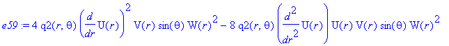


![]()
and taking into account the form of metric:
| > | e60 := coeff(rhs(logunov),dt^2 ); e61 := subs( `r*`=r,coeff(rhs(logunov),d(`r*`)^2 ) ); e62 := subs( `r*`=r,coeff(rhs(logunov),d(theta)^2 ) ); e63 := subs( `r*`=r,coeff(rhs(logunov),d(phi)^2 ) ); subs( {U(r)=epsilon/2,V(r) = r^2/2/Delta(r),W(r) = r},e59 ):# U=e60, Delta(r)=r^2*(1-1/r), `h*`=c=G=1,W=r,rg=2*M/c^2=1 numer( simplify(%) ): e64 := expand(-%/(r^4*epsilon^2)); |
![]()
![]()


![]()
To simplify this equation let us consider the parts with and without derivatives of the perturbation functions separately.
| > | # part with derivatives e65 := -diff(q2(r,theta),`$`(theta,2))*sin(theta) - 3*cos(theta)*diff(q2(r,theta),theta) + 3*cos(theta)*diff(q3(r,theta),r) + diff(q3(r,theta),r,theta)*sin(theta); |

| > | # part without derivatives e66 := e64 - e65; |

![]()
From the latter expression we have:
| > | subs( Delta(r)=r^2*(1-1/r),e66 ): factor(%)/(q2(r,theta)*sin(theta)): e67 := expand(%)*q2(r,theta)*sin(theta); |

or
| > | 4*r^4*epsilon-4*r^3*epsilon-4*r^4*epsilon*cos(theta)^2+4*r^3*epsilon*cos(theta)^2; simplify(%); 4*epsilon*r^4*sin(theta)^2*(1 - 1/r); simplify(% - %%);# verification |
![]()
![]()
![]()
![]()
Hence the part without derivatives of the perturbation functions is:
| > | e68 := ( -2 + 6/r - 2*sigma^2*r^2/epsilon + 4*epsilon*r^4*sin(theta)^2*(1-1/r) )*q2(r,theta)*sin(theta); subs( Delta(r)=r^2*(1-1/r),% ): simplify( e67 - % );# verification |
![]()
As a result, the complete equation has a form:
| > | e69 := e65 + e68; |

Let us introduce new function:
| > | fun := Q(r,theta) = (diff(q3(r,theta),r) - diff(q2(r,theta),theta))*sin(theta)^3; |
![]()
Now we can replace the part of the equation containing the derivatives of the perturbation functions by:
| > | F1 := Diff( Q(r,theta),theta )/sin(theta)^2;# new function expand( value(subs(Q(r,theta)=rhs(fun),F1)) - e65); |
![]()
Thus, the resulting equation has a form:
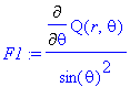
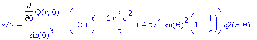
| > | e70 := F1/sin(theta) + e68/sin(theta); |
Now we shall perform the similar manipulation with the second equation governing the axial perturbations.
| > | get_compts( Lgvp )[3,4]: simplify( subs({f1,f2,f4},%) ): e71 := expand( 4*numer(%)/delta/exp(sigma*t*I) ); |
![]()


![]()
Taking into account the metric we have
| > | subs( {U(r)=epsilon/2,V(r) = r^2/2/Delta(r),W(r) = r},e71 ): numer( simplify(%) ): e72 := expand(-%/r^3/epsilon); |


Let us transform the part of this equation containing the derivatives of perturbation functions.
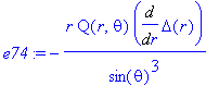
| > | e73 := -2*Delta(r)*r*Diff( Q(r,theta),r )/sin(theta)^3; subs(Q(r,theta)=rhs( fun ),%): expand(value(%)); |
| > | e74 := -r*Q(r,theta)*Diff(Delta(r),r)/sin(theta)^3; subs(Q(r,theta)=rhs( fun ),%): expand(value(%)); |
![]()
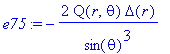
| > | e75 := -2*Q(r,theta)*Delta(r)/sin(theta)^3; subs(Q(r,theta)=rhs( fun ),%): expand(value(%)); |
![]()
Resulting expression for this part is:
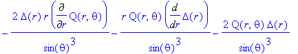
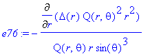
| > | e73 + e74 + e75; e76 := -Diff(Delta(r)*Q(r,theta)^2*r^2,r)/Q(r,theta)/r/sin(theta)^3; expand( value(%) ); |
Part without derivatives is:
| > | e77 := (-2*sigma^2/epsilon + 2*epsilon*sin(theta)^2)*r^3*q3(r,theta); |
Thus, the final expression is:
| > | e78 := e76 + e77; |
| > | # verification simplify( subs({Q(r,theta)=rhs(fun),Delta(r)=r^2*(1-1/r)},e78 - e72) ); |
![]()
Thus, we have two equations for the perturbation functions:
| > | # Thus eq[25] := e70 = 0; eq[26] := e78 = 0; |
![eq[25] := Diff(Q(r,theta),theta)/sin(theta)^3+(-2+6/r-2*r^2/epsilon*sigma^2+4*epsilon*r^4*sin(theta)^2*(1-1/r))*q2(r,theta) = 0](images/rtg_bh391.gif)
![eq[26] := -Diff(Delta(r)*Q(r,theta)^2*r^2,r)/Q(r,theta)/r/sin(theta)^3+(-2*sigma^2/epsilon+2*epsilon*sin(theta)^2)*r^3*q3(r,theta) = 0](images/rtg_bh392.gif)
In order to reduce this system to a single equation let us introduce two functions:
| > | e79 := A(r,theta) = coeff( lhs(eq[25]),q2(r,theta) ); e80 := op( 1,lhs(eq[25]) )/lhs(e79) + q2(r,theta); e81 := B(r,theta) = coeff( lhs(eq[26]),q3(r,theta) ); e82 := op( 1,lhs(eq[26]) )/lhs(e81) + q3(r,theta); |
Hence we can reduce the obtain system to the second-order equation for
![]() .
.
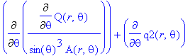
| > | Diff(op(1,e82),r) + diff(op(2,e82),r); Diff(op(1,e80),theta) + diff(op(2,e80),theta); e83 := %% - %; fun; |
![]()
To avoid trivializing the eigenfunction problem let us made some transformation of the obtained equation ( n is some number):
| > | # Hence eq[27] := op(1,e83) + op(3,e83) + (n+1)*Q(r,theta)/sin(theta)^3 = n*Q(r,theta)/sin(theta)^3; |
![eq[27] := Diff(-Diff(Delta(r)*Q(r,theta)^2*r^2,r)/Q(r,theta)/r/sin(theta)^3/B(r,theta),r)-Diff(Diff(Q(r,theta),theta)/sin(theta)^3/A(r,theta),theta)+(n+1)*Q(r,theta)/sin(theta)^3 = n*Q(r,theta)/sin(the...](images/rtg_bh402.gif)
We can eliminate the
![]() -dependence from A and B as
-dependence from A and B as
![]() is extremely small value (see above):
is extremely small value (see above):
| > | e84 := `A*`(r) = rhs(e79) - op(4,rhs(e79)); expand(e81): e85 := `B*`(r) = op(1,rhs(%)); |
Now we can separate variables:
| > | value( subs( {A(r,theta)=`A*`(r),B(r,theta)=`B*`(r),Q(r,theta)= Xi(r)*Upsilon(theta)},eq[27])):# Q(r,theta) = Xi(r)*Upsilon(theta) e86 := expand(%*sin(theta)^3*`A*`(r)/Xi(r)); |


Hence:
| > | e84; eq[28] := diff(Upsilon(theta),`$`(theta,2)) - 3/sin(theta)*diff(Upsilon(theta),theta)*cos(theta) + 2*n*Upsilon(theta) = 0; lhs(e86) + op(1,lhs(eq[28])) + op(2,lhs(eq[28])) - `A*`(r)*n*Upsilon(theta) + ( op(2,rhs(e84)) + op(3,rhs(e84)))*n*Upsilon(theta) = rhs(e86): e87 := expand(%/Upsilon(theta)*Xi(r)/`A*`(r)/2); |
![eq[28] := diff(Upsilon(theta),`$`(theta,2))-3/sin(theta)*diff(Upsilon(theta),theta)*cos(theta)+2*n*Upsilon(theta) = 0](images/rtg_bh411.gif)

As it takes a place in the case of the Schwarzschild black hole,
![]() is the Gegenbauer's equation and can be solved through
Legendre functions (see
S. Chandasekhar, "
The mathematical theory of black holes
", Clarendon Press, 1983, Ch. 4
)
:
is the Gegenbauer's equation and can be solved through
Legendre functions (see
S. Chandasekhar, "
The mathematical theory of black holes
", Clarendon Press, 1983, Ch. 4
)
:
| > | dsolve(eq[28],Upsilon(theta)); |
![]()
![]()
As their degree is integer-valued we have ( l is integer):
| > | n = factor( solve( 1/2*(9+8*n)^(1/2)-1/2 = l,n ) ); |
![]()
The part of the "radial" equation e87 containing the derivatives of the unknown function can be transformed in the following way:
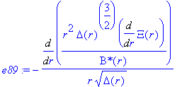
| > | e88 := -3/2*r/`B*`(r)*diff(Delta(r),r)*diff(Xi(r),r) - 2/`B*`(r)*Delta(r)*diff(Xi(r),r) - r/`B*`(r)*Delta(r)*diff(Xi(r),`$`(r,2)) + r/`B*`(r)^2*diff(`B*`(r),r)*Delta(r)*diff(Xi(r),r); e89 := -Diff(r^2*Delta(r)^(3/2)*Diff(Xi(r),r)/`B*`(r),r)/(r*sqrt(Delta(r))); simplify(e88 - value(e89));# verification |
![]()
Then the equation for the radial function takes a form:
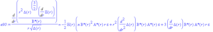
| > | e90 := -e89 = -simplify( rhs(e87) - (lhs(e87) - e88)); simplify( ( lhs(e87) - rhs(e87) ) + ( value(lhs(%)) - rhs(%) ) );# verification |

![]()
![]()
Its right-hand side is
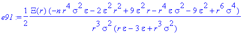
| > | subs( {e84,e85,Delta(r)=r^2*(1-1/r)},rhs(e90) ): e91 := simplify(%); |
and the left-hand side is
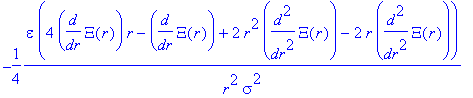
| > | subs( {e85,Delta(r)=r^2*(1-1/r)},lhs(e90) ): simplify(value(%)); |
Collecting of derivatives results in
| > | e92 := Diff(2*Delta(r)*diff(Xi(r),r),r) + diff(Xi(r),r) = e91*(-4*r^2*sigma^2/epsilon); expand(value(subs(Delta(r)=r^2*(1-1/r),lhs(%))));# verification of the left-hand side |

Since
![]() is small value, we can expand the right-hand side and omit the terms which are proportional to
is small value, we can expand the right-hand side and omit the terms which are proportional to
![]() (
k
is some positive number):
(
k
is some positive number):
| > | series(rhs(e92),epsilon); convert(%,polynom); e93 := op(1,%) + op(2,%); |

As a result, we obtain
| > | eq[29] := lhs(e92) = simplify( e93 ); |
![eq[29] := Diff(2*Delta(r)*diff(Xi(r),r),r)+diff(Xi(r),r) = -2*Xi(r)/r*(r^3*sigma^2-epsilon*r*n-2*r*epsilon+3*epsilon)/epsilon](images/rtg_bh436.gif)
or otherwise
| > | simplify(subs(Delta(r)=r^2*(1-1/r),eq[29])): r*epsilon*lhs(%) - rhs(%)*r*epsilon: e94 := collect(%,{diff(Xi(r),`$`(r,2)),diff(Xi(r),r)}); |

Since
![]() ~
~
 in the vicinity of the singularity (see numerical consideration above), we can omit the first term in
![]() . This approximation means also that we can consider
. This approximation means also that we can consider
![]() outside its extremum. Thus
outside its extremum. Thus
| > | e95 := r*epsilon*(4*r-1)*diff(Xi(r),r) + 2*Xi(r)*(r^3*sigma^2-epsilon*r*n-2*r*epsilon+3*epsilon);# e94 |
![]()
| > | sol1 := dsolve(e95,Xi(r)); |
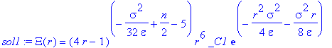
If we rewrite
r
=
![]() , then the solution takes a simple form:
, then the solution takes a simple form:
| > | subs(r=1+epsilon*x,rhs(sol1)): simplify(%); |
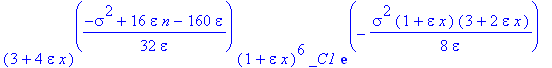
This simple solution suggests: 1) extremum, which is defined by the first term, appears due to growing angular number
l
; 2) appropriate asymptotical behavior, which is defined by the exponentially decaying second term, corresponds only to
![]() >0. Since
>0. Since
![]() <0 would result in the time-growing perturbations, we can conclude that the investigated metrics is
stable
. The stability far from the singularity, where the metric coincides with the Schwarzschild one, is provided by the stability of the latter.
<0 would result in the time-growing perturbations, we can conclude that the investigated metrics is
stable
. The stability far from the singularity, where the metric coincides with the Schwarzschild one, is provided by the stability of the latter.
The form of the perturbations can be obtained in the following way.
![]() and
and
![]() give
give
![]() . On the other hand, from
. On the other hand, from
![]() we have:
we have:
| > | eq[24]; e96 := collect( subs(rg=1,%),{diff(q2(r,theta),r),q2(r,theta)} ); |
![]()
![]()
Then
| > | Q(r,theta) = (diff(q3(r,theta),r)-diff(q2(r,theta),theta))*sin(theta)^3; e97 := diff(q3(r,theta),r) = solve(%,diff(q3(r,theta),r)); diff(lhs(e96),r): subs(e97,%): numer( simplify(%) ): collect(%,{diff(q2(r,theta),`$`(r,2)),diff(q2(r,theta),r),diff(q2(r,theta),`$`(theta,2)),diff(q2(r,theta),theta)}); |
![]()


![]()
The solution of the latter would give
![]() and, as a consequence, we can find
and, as a consequence, we can find
![]() as well.
as well.
Conclusion and outlook
The non-zero mass of graviton in the RTG causes the strong repulsion within the sub-Planckian distances for the collapsing stellar objects. As a result, the final stage of the collapse requires a quantum-field investigation. We can surmise that this stage entails the transformation of the matter into the gravitational radiation, that is gravitational explosion of the stellar remainder. It is surprisingly, but the strong repulsion in the vicinity of the Schwarzschild singularity does not result in the destabilization of the vacuum spherically symmetric solution in the RTG. Nevertheless, this stable solution is physically unreachable due to the graviton induced repulsion (in the correspondence with the causality principle in the RTG).
Thus, the statement about the absence of the physical singularity in the RTG needs a further validation because of it appeals to the sub-Planckian physics (at least in the case of the stellar object collapse). Apparently, only a quantization of the gravitational field will allow understanding the final stages of the massive star evolution.
� V.L.Kalashnikov, 04-21-2003