Cosmological models in the relativistic theory of gravitation
by Vladimir Kalashnikov
Abstract : We present the reproduction of the calculations describing the cosmological models in the so-called Relativistic Theory of Gravity (RTG). This theory is the alternative to the General theory of Relativity (GR) and supposes the field (non geometrical) character of the gravitation. The logicality of its intrinsic assumptions inspires to consider the experimental consequences of RTG. Basic references are A.A. Logunov, Relativistic theory of gravity , Nova Sc. Publications (1998) and A.A. Logunov, M.A. Mestvirishvili, Relativistic theory of gravity , Moskow, Nauka (1989, in Russian). We expect, that the computer algebra algorithmization will promote the investigations and discussions in this field. As the development of the model aimed at the explanation of the accelerated expansion of the universe, we consider the universe evolution in framework of RTG. Such development is based on the introduction of the generalized dark matter (X-matter) and tacking into account the causality principle.
Introduction (basic equations)
Briefly the basic postulate of RTG is the existence of the flat pseudo-Euclidian background metrics
![]() in compliance with the special relativity. This allows to keep a law of the energy-momentum conservation. The gravitation is the tensor field with spin 2, which influences on the energy-momentum of matter defined by a tensor
in compliance with the special relativity. This allows to keep a law of the energy-momentum conservation. The gravitation is the tensor field with spin 2, which influences on the energy-momentum of matter defined by a tensor
![]() . The source of this field is also
. The source of this field is also
![]() . Hence, the universal and tensor character of the gravitation allows to introduce the effective Riemannian spacetime with the metrics
. Hence, the universal and tensor character of the gravitation allows to introduce the effective Riemannian spacetime with the metrics
![]() on the flat background. This effective spacetime has only dynamical sense and allows to refer to flat background at any moment. This overcomes the uncertainty in the coordinate choice in GR. The tensor density for the metrics of the effective curved spacetime
on the flat background. This effective spacetime has only dynamical sense and allows to refer to flat background at any moment. This overcomes the uncertainty in the coordinate choice in GR. The tensor density for the metrics of the effective curved spacetime
![]() (avoid the mishmash with the Einstein's tensor!) is:
(avoid the mishmash with the Einstein's tensor!) is:
![]() =
=
![]()
![]() =
=
![]()
![]() +
+
![]()
![]() ,
,
where
![]() is the tensor of the gravitational field. The field equations are:
is the tensor of the gravitational field. The field equations are:
![]() -
-
![]()
![]() R
= - 8
R
= - 8
![]()
![]() ,
,
![D[m]*G^mn = 0](images/rtg119.gif) ,
,
where
![]() is the covariant derivative on the background metrics. The first equation is the usual Einstein-Hilbert's equation, the second equation removes the states with the spin 0 and 1 and keeps the background metrics in the field equations. In this case, all variables depend on the background metrics.
is the covariant derivative on the background metrics. The first equation is the usual Einstein-Hilbert's equation, the second equation removes the states with the spin 0 and 1 and keeps the background metrics in the field equations. In this case, all variables depend on the background metrics.
Homogeneous and isotropic universe
The effective Riemannian homogeneous and isotropic spacetime can be described by an interval (signature -2, spherical coordinates):
 .
.
The corresponding metrics is:
>
restart:
with(tensor):
with(linalg):
with(DEtools):
with(plots):
coord := [t, r, theta, phi]:# spherical coordinates
g_compts := array(symmetric,sparse,1..4,1..4):
g_compts[1,1] := U(t,r):#dt^2
g_compts[2,2] := -V(t,r):#dr^2
g_compts[3,3]:= -W(t,r):#dtheta^2
g_compts[4,4]:=-W(t,r)*sin(theta)^2:#dphi^2
g := create([-1,-1], eval(g_compts));# covariant components of metrics
ginv := invert( g, 'detg' ):
g_scal := det(get_compts(g));# scalar of metrics tensor
Warning, the protected names norm and trace have been redefined and unprotected
Warning, the name adjoint has been redefined
Warning, the name changecoords has been redefined
![g := TABLE([index_char = [-1, -1], compts = matrix(...](images/rtg122.gif)
![]()
As a source, we will use the energy-momentum tensor for the perfect liquid:
![]() .
.
In the concomitant coordinates
![]() =0 (
m
=1, 2, 3, 4;
=0 (
m
=1, 2, 3, 4;
![]() =1, 2, 3) and, as
=1, 2, 3) and, as
![g[mn]*u^m*u^n = 1](images/rtg127.gif) (hence
(hence
![]() =
=
![]() ), then we have:
), then we have:
>
T_compts := array(symmetric,sparse,1..4,1..4):# energy-momentum tensor components
T_compts[1,1] := U(t,r)*rho(t):
T_compts[2,2] := V(t,r)*p(t):
T_compts[3,3] := W(t,r)*p(t):
T_compts[4,4] := W(t,r)*sin(theta)^2*p(t):
T := create([-1,-1], eval(T_compts));# covariant energy-momentum tensor
![T := TABLE([index_char = [-1, -1], compts = matrix(...](images/rtg130.gif)
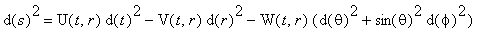
For the beginning, we consider the covariant conservation law:
![]() [;
n
]= 0, where [;
n
] denotes the covariant derivative on the Riemannian metrics and
[;
n
]= 0, where [;
n
] denotes the covariant derivative on the Riemannian metrics and
![T[m]^n = (rho(t)+p(t))*u[m]*u^n-delta[m]^n*p(t)](images/rtg132.gif) .
.
>
T_compts := array(symmetric,sparse,1..4,1..4):# energy-momentum tensor components
T_compts[1,1] := rho(t):
T_compts[2,2] := -p(t):
T_compts[3,3] := -p(t):
T_compts[4,4] := -p(t):
TT := create([-1,1], eval(T_compts));# [-1,1] energy-momentum tensor
![TT := TABLE([index_char = [-1, 1], compts = matrix(...](images/rtg133.gif)
>
d1g:= d1metric(g, coord):# covariant derivative
Cf1:= Christoffel1 ( d1g ):
Cf2:= Christoffel2 ( ginv, Cf1 ):
Z := cov_diff( TT, coord, Cf2 ):
ZZ := contract(Z,[2,3]);
![]()
![ZZ := TABLE([index_char = [-1], compts = vector([1/...](images/rtg135.gif)
![]()
![ZZ := TABLE([index_char = [-1], compts = vector([1/...](images/rtg137.gif)
![]()
> get_compts(ZZ)[2] = 0;
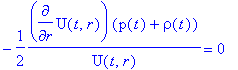
Hence
 = 0 if
![]() +
+
![]() is not equal to 0. The second equation is:
is not equal to 0. The second equation is:
> expand( get_compts(ZZ)[1] ) = 0;
It is obviously, that this expression can be rewritten as:
> eq1 := diff(rho(t),t) = -Diff(ln(sqrt(V(t,r))*W(t,r)),t)*(p(t)+rho(t));
![]()
Now we consider the second group of the field equation. Let's find
![]()
>
G_compts := array(symmetric,sparse,1..4,1..4):
G_compts[1,1] := simplify( sqrt(-g_scal)*get_compts(ginv)[1,1],radical,symbolic ):#dt^2
G_compts[2,2] := simplify( sqrt(-g_scal)*get_compts(ginv)[2,2],radical,symbolic ):#chi^2
G_compts[3,3]:= simplify( sqrt(-g_scal)*get_compts(ginv)[3,3],radical,symbolic ):#dtheta^2
G_compts[4,4]:= simplify( sqrt(-g_scal)*get_compts(ginv)[4,4],radical,symbolic ):#dphi^2
G := create([1,1], eval(G_compts));# contravariant components of G
![]()
![G := TABLE([index_char = [1, 1], compts = matrix([[...](images/rtg147.gif)
![]()
and define the background metrics
![]()
>
mu_compts := array(symmetric,sparse,1..4,1..4):
mu_compts[1,1] := 1:#dt^2
mu_compts[2,2] := -1:#chi^2
mu_compts[3,3]:= -r^2:#dtheta^2
mu_compts[4,4]:= -r^2*sin(theta)^2:#dphi^2
mu := create([-1,-1], eval(mu_compts));# covariant components of mu
muinv := invert( mu, 'detg' ):
![mu := TABLE([index_char = [-1, -1], compts = matrix...](images/rtg150.gif)
Now, we are able to calculate
![D[m]*G^mn](images/rtg151.gif) . But the direct calculation by the standard procedure
cov_diff
does not give a correct result (!?):
. But the direct calculation by the standard procedure
cov_diff
does not give a correct result (!?):
>
d1mu:= d1metric(mu, coord):
Cf1:= Christoffel1 ( d1mu ):
Cf2:= Christoffel2 ( muinv, Cf1 ):
Z := cov_diff( G, coord, Cf2 ):
contract(Z,[1,3]);
![]()
![TABLE([index_char = [1], compts = vector([1/2*sin(t...](images/rtg153.gif)
![]()
![TABLE([index_char = [1], compts = vector([1/2*sin(t...](images/rtg155.gif)
![]()
The error becomes apparent by the appearance of the unnatural condition
![]() = 0. The correct result can be obtained by the direct calculation
= 0. The correct result can be obtained by the direct calculation
![D[m]*G^mn](images/rtg158.gif) =
=
![diff(G^mn,x[m])+Gamma[pm]^n*G^mp](images/rtg159.gif) = 0:
= 0:
>
A1 := partial_diff( G, coord ):
A2 := contract(A1,[2,3]):
d1mu:= d1metric(mu, coord):
Cf1:= Christoffel1 ( d1mu ):
Cf2:= Christoffel2 ( muinv, Cf1 ):
ZZZ := prod(Cf2,G):
A3 := contract(ZZZ,[2,5] ):
A4 := contract(A3,[2,3]):
e1 := simplify(get_compts(A2)[1] + get_compts(A4)[1]);
e2 := simplify(get_compts(A2)[2] + get_compts(A4)[2]);
simplify(get_compts(A2)[3] + get_compts(A4)[3]);

![]()
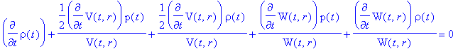
The first obtained equation is:
> expand(numer( e1 )/sin(theta)/2) = 0;
![]()
This equation can be rewritten as:
>
eq2 := Diff(sqrt(V(t,r)/U(t,r))*W(t,r),t) = 0;
print(`check-up:`);
expand(numer(simplify( diff(sqrt(V(t,r)/U(t,r))*W(t,r),t) ))/2);
![]()
![]()
![]()
The second obtained equation is:
> expand(numer( e2 )/(-2*sin(theta))) = 0;
![]()
Hence
>
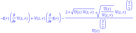
eq3 := Diff(sqrt(U(t,r)/V(t,r))*W(t,r),r) = 2*r*sqrt(U(t,r)*V(t,r));
print(`check-up:`);
expand(numer(simplify( value(lhs(eq3)) - rhs(eq3) ))/2);
![]()
![]()
![]()
From eq2 we have
>
simplify( int(lhs(eq2),t)*sqrt(U(t,r)),sqrt ) = sqrt(U(t,r))*f(t);
# or
eq4 := sqrt(V(t,r))*W(t,r)=sqrt(U(t,r))*f(r);
![]()
![]()
and, as a result, eq1 gives:
> eq5 := subs(sqrt(V(t,r))*W(t,r)=sqrt(U(t,r)),eq1);# as Diff(ln(sqrt(U(t,r))*f(t)),t) = Diff(ln(sqrt(U(t,r)),t) + Diff(f(r),t) = Diff(ln(sqrt(U(t,r)),t)
![]()
So, the obtained on this stage result can be written in the following way:
>
print(`The result obtained from the covariant conservation law and second field equation:`);
Diff(U(t,r),r) = 0;
fun[1] := subs(U(t,r)=U(t),eq5);
fun[2] := subs(U(t,r)=U(t),eq4);
fun[3] := subs(U(t,r)=U(t),eq3);
![]()
![]()
![]()
![]()
![]()
The manipulations with
![]() and
and
![]() results in:
results in:
>
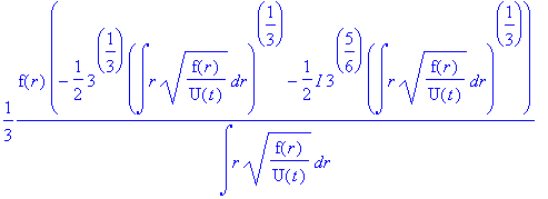
simplify(value(lhs(fun[3])) - rhs(fun[3])):
subs(W(t,r)=solve(fun[2],W(t,r)),numer(%)):
simplify(%):
expand( numer(%)/(2*U(t)^(3/2)) );
>
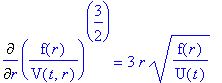
# or
eq6 := Diff(f(r)/V(t,r),r) = 2*r*sqrt(V(t,r)/U(t));# because of Diff(f(r)/V(t,r),r) = (-f(r)*diff(V(t,r),r)+V(t,r)*diff(f(r),r))/V(t,r)^2
![]()
Now
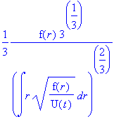
> simplify( eq6*sqrt(f(r)/V(t,r)) );
![]()
>
#or
Diff((f(r)/V(t,r))^(3/2),r) = 3*r*sqrt(f(r)/U(t));
>
int(lhs(%),r) = int(rhs(%),r);
solve(%,V(t,r));
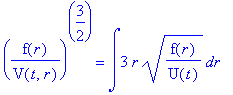
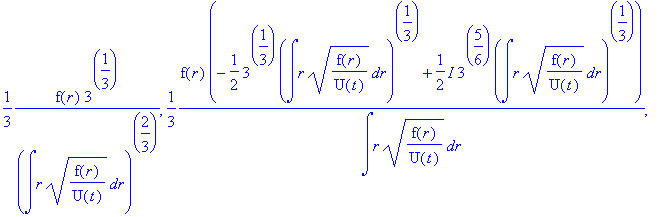
> %[1];
>
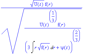
# Hence
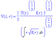
fun[4] := V(t,r) = sqrt(U(t))^(2/3)*f(r)/(3*Int(r*sqrt(f(r)),r) + psi(t))^(2/3);# here psi(t) is arbitrary function of t
![fun[4] := V(t,r) = U(t)^(1/3)*f(r)/((3*Int(r*sqrt(f...](images/rtg189.gif)
> simplify( subs( V(t,r)=rhs(fun[4]),solve(fun[2],W(t,r)) ) );# from fun[4] and fun[2] for W
>
# or
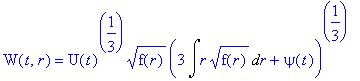
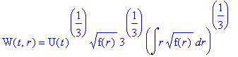
fun[5] := W(t,r) = U(t)^(1/3)*sqrt(f(r))*(3*Int(r*sqrt(f(r)),r)+psi(t))^(1/3);
![fun[5] := W(t,r) = U(t)^(1/3)*sqrt(f(r))*(3*Int(r*s...](images/rtg191.gif)
Let's draw attention on the Einstein-Hilbert's equations:
>
D1g := d1metric( g, coord ):
D2g := d2metric( D1g, coord ):
Cf1 := Christoffel1 ( D1g ):
RMN := Riemann( ginv, D2g, Cf1 ):
RICCI := Ricci( ginv, RMN ):
RS := Ricciscalar( ginv, RICCI ):
Ein := act( subs,U(t,r)=U(t),Einstein( g, RICCI, RS ) ):# Einstein tensor
displayGR(Einstein,Ein);#non-zero components of Einstein tensor
![]()
![]()


![]()
Hilbert-Einstein's equations:
>
E[1] := numer(simplify( get_compts(Ein)[1,1] + 8*Pi*get_compts(T)[1,1] ));
E[2] := numer(simplify( get_compts(Ein)[1,2] ));
E[3] := numer(simplify( get_compts(Ein)[2,2] + 8*Pi*get_compts(T)[2,2] ));
E[4] := numer(simplify( get_compts(Ein)[3,3] + 8*Pi*get_compts(T)[3,3] ));
E[5] := expand(numer(simplify( get_compts(Ein)[4,4] + 8*Pi*get_compts(T)[4,4] ))/(-1+cos(theta)^2));
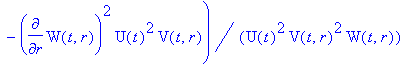
![E[1] := -diff(W(t,r),t)^2*V(t,r)^2-diff(W(t,r),r)^2...](images/rtg1111.gif)
![]()
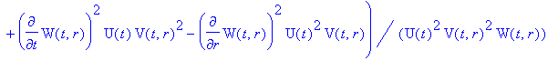
![E[2] := 2*diff(W(t,r),r,t)*V(t,r)*W(t,r)-diff(V(t,r...](images/rtg1113.gif)
![E[3] := 4*diff(W(t,r),`$`(t,2))*U(t)*V(t,r)*W(t,r)-...](images/rtg1114.gif)
![]()
![E[4] := 2*diff(W(t,r),`$`(t,2))*U(t)*V(t,r)^2*W(t,r...](images/rtg1116.gif)
![E[4] := 2*diff(W(t,r),`$`(t,2))*U(t)*V(t,r)^2*W(t,r...](images/rtg1117.gif)
![E[4] := 2*diff(W(t,r),`$`(t,2))*U(t)*V(t,r)^2*W(t,r...](images/rtg1118.gif)
![]()
![E[5] := -2*diff(W(t,r),`$`(t,2))*U(t)*V(t,r)^2*W(t,...](images/rtg1120.gif)
![E[5] := -2*diff(W(t,r),`$`(t,2))*U(t)*V(t,r)^2*W(t,...](images/rtg1121.gif)
![E[5] := -2*diff(W(t,r),`$`(t,2))*U(t)*V(t,r)^2*W(t,...](images/rtg1122.gif)
![]()
Two latter two equations are identical:
> simplify(E[4]+E[5]);
![]()
Let's consider second equation:
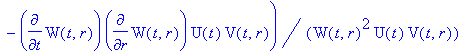
> expand( E[2]/(-2*V(t,r)*W(t,r)) ) = 0;
and make some manipulations:
> expand( lhs(%/(-diff(W(t,r),r))) ) = 0;
>
# Hence
Diff( ln(Diff(W(t,r),r)/sqrt(V(t,r)*W(t,r))),t ) = 0;
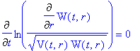
As a consequence
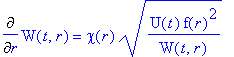
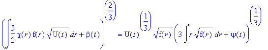
> eq7 := Diff(W(t,r),r) = chi(r)*sqrt(V(t,r)*W(t,r));# chi(r) is arbitrary function of r
![]()
On the other hand, as
>
lhs(fun[4])*lhs(fun[5])^2 = rhs(fun[4])*rhs(fun[5])^2;
solve(%,V(t,r));
![]()

>
# Hence
subs(V(t,r)=%,eq7);
>
# and
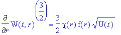
Diff(W(t,r)^(3/2),r) = (3/2)*chi(r)*f(r)*sqrt(U(t));
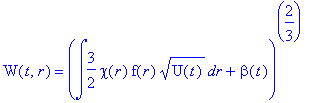
As a result:
> W(t,r) = ( int(rhs(%),r) + beta(t) )^(2/3);# beta(t) is the arbitrary function of t
>
# Let's compare with
fun[5];
So, we have
> rhs(%%) = rhs(%);
This results in
![]() =
=
![]() = 0 and
= 0 and
> fun[6] := Int(chi(r)*f(r),r) = 2/3*f(r)^(3/4)*sqrt(3*Int(r*sqrt(f(r)),r));
![fun[6] := Int(chi(r)*f(r),r) = 2/3*f(r)^(3/4)*sqrt(...](images/rtg1138.gif)
This equation allows to define
![]() . Now from
. Now from
![]() and
and
![]() :
:
>
subs(psi(t)=0,fun[4]);
subs(psi(t)=0,fun[5]);
# or
fun[7] := V(t,r) = U(t)^(1/3)*P(r);# P(r) = 1/3*f(r)*3^(1/3)/(Int(r*sqrt(f(r)),r)^(2/3))
fun[8] := W(t,r) = U(t)^(1/3)*R(r);# R(r) = sqrt(f(r))*3^(1/3)*Int(r*sqrt(f(r)),r)^(1/3)
![fun[7] := V(t,r) = U(t)^(1/3)*P(r)](images/rtg1144.gif)
![fun[8] := W(t,r) = U(t)^(1/3)*R(r)](images/rtg1145.gif)
Then from
![]() :
:
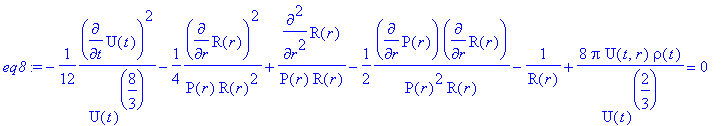
> eq8 := expand(subs({V(t,r)=rhs(fun[7]),W(t,r)=rhs(fun[8])},E[1])/(P(r)*R(r))^2/U(t)^2/4) = 0;
And from
![]() :
:
> eq9 := expand(subs({V(t,r)=rhs(fun[7]),W(t,r)=rhs(fun[8])},E[3])/R(r)^2/4/P(r)/U(t)^(8/3)) = 0;
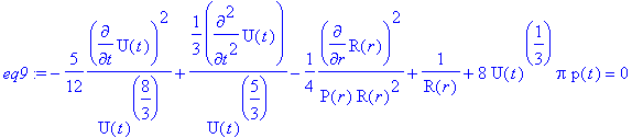
eq8 and eq9 can be regrouped as:
>
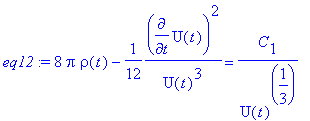
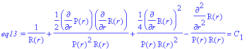
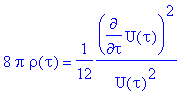
eq10 := U(t)^(1/3)*(8*pi*rho(t) - 1/12*diff(U(t),t)^2/U(t)^3) = 1/R(r) + 1/2*diff(P(r),r)*diff(R(r),r)/(P(r)^2*R(r)) + 1/4*diff(R(r),r)^2/(P(r)*R(r)^2) - diff(R(r),`$`(r,2))/(P(r)*R(r));
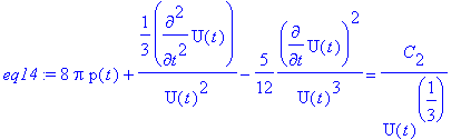
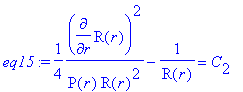
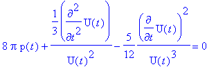
eq11 := U(t)^(1/3)*(8*Pi*p(t) + 1/3*diff(U(t),`$`(t,2))/U(t)^2 - 5/12*diff(U(t),t)^2/U(t)^3) = 1/4*diff(R(r),r)^2/(P(r)*R(r)^2) - 1/R(r);
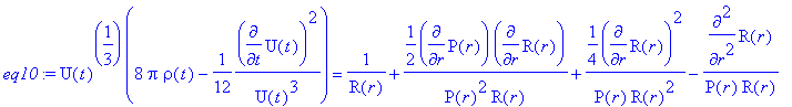
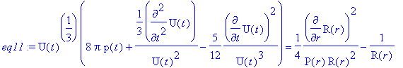
As the left-hand sides depend only on t and the right-hand side depend only on r , we can write:
>
eq12 := lhs(eq10)/U(t)^(1/3) = C[1]/U(t)^(1/3);# C[1] is a constant
eq13 := rhs(eq10) = C[1];
# and
eq14 := lhs(eq11)/U(t)^(1/3) = C[2]/U(t)^(1/3);# C[2] is a constant
eq15 := rhs(eq11) = C[2];
The next manipulation with obtained expressions gives the connection between the constants:
>
eq16 := solve(eq15,P(r));# solution for P(r)
simplify( subs(P(r)=%,eq13) );
![eq16 := 1/4*diff(R(r),r)^2/(R(r)*(1+C[2]*R(r)))](images/rtg1156.gif)
![]()
As it follows from the previous substitution:
>
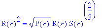
eq17 := P(r) = f(r)/S(r)^(2/3);# S(r) = 3*Int(r*sqrt(f(r)),r)
eq18 := R(r)^2 = f(r)*S(r)^(2/3);
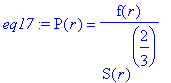

>
lhs(eq17)*lhs(eq18) = rhs(eq17)*rhs(eq18);
fun[9] := f(r) = solve(%,f(r))[1];
![]()
![]()
>
subs(f(r)=rhs(fun[9]),eq18);
fun[10] := S(r) = solve(%,S(r))[1];
![fun[10] := S(r) = sqrt(sqrt(P(r))*R(r))*R(r)/P(r)](images/rtg1163.gif)
For the last expression:
>
subs(S(r) = 3*Int(r*sqrt(f(r)),r),lhs(fun[10])) = rhs(fun[10]):
simplify( diff(%,r) ):
simplify( subs(f(r)=rhs(fun[9]),%)/(3*sqrt(sqrt(P(r))*R(r))) );
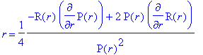
Since
 , the last expression can be rewritten:
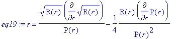
> eq19 := r = sqrt(R(r))*Diff(sqrt(R(r)),r)/P(r) - R(r)*Diff(P(r),r)/P(r)^2/4;
Likewise for eq16 we have:
> eq20 := P(r) = Diff(sqrt(R(r)),r)^2/(1+C[2]*R(r));
![eq20 := P(r) = Diff(sqrt(R(r)),r)^2/(1+C[2]*R(r))](images/rtg1167.gif)
>
subs(P(r)=rhs(eq20),eq19);
subs(R(r)=x(r)^2,subs(sqrt(R(r))=x(r),%)):# x(r)=sqrt(R(r))
simplify(value(%));
![r = sqrt(R(r))*(1+C[2]*R(r))/Diff(sqrt(R(r)),r)-1/4...](images/rtg1168.gif)
![r = 1/2*(2*diff(x(r),r)^2+3*diff(x(r),r)^2*C[2]*x(r...](images/rtg1169.gif)
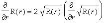
Now we transit to new variable
x=
![]() so that
r
=
r
(
x
). As
dr
=
so that
r
=
r
(
x
). As
dr
=
 ,
,
 and
and

![]()
![]() =
=
 , the latter obtained solution can be transformed:
> eq21 := x^2*(C[2]*x^2 + 1)*Diff(r(x),x$2) + x*(3*C[2]*x^2 + 2)*Diff(r(x),x) -2*r(x) = 0;
![eq21 := x^2*(C[2]*x^2+1)*Diff(r(x),`$`(x,2))+x*(3*C...](images/rtg1177.gif)
>
simplify(subs(C[2]=C,eq21)):
assume(C>=0):
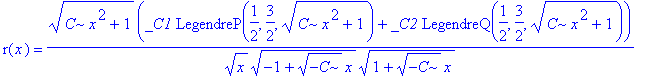
simplify(dsolve(%,r(x)),radical,symbolic);
>
assume(C<0):
simplify(subs(C[2]=C,eq21)):
simplify(dsolve(%,r(x)),radical,symbolic);
It should be noted, that Mathematica gives straight away the simplified result through elementary functions:
>
C := 'C':
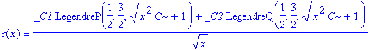
r(x) = C_1/x^2 + C_2*(sqrt(C*(1+C*x^2))*x - arcsinh(x*sqrt(C)))/x^2;
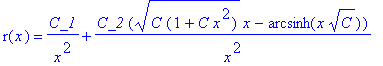
> convert(%,ln);
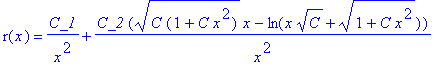
We take only solutions, which provide for the trivial topology because the Riemannian metrics coefficients are the functions of the Minkowski spacetime coordinates. The spherical Riemannian spacetime can not be covered by the single flat chart and must be rejected. So, we search the continuous, one-to-one and codirectional dependences of r on x . This can be satisfied only by C =0
>
simplify(subs(C[2]=0,eq21)):
expand(dsolve(%,r(x)));
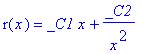
and _C2 =0
> eq22 := subs(_C2=0,%);
![]()
Now let's remember
eq12
and
eq14
. Since
![]() =
=
![]() =0 as a result of the existence of the background metrics with trivial topology, the matter defines only
U
but not
P
and
R
. Therefore
_C1
does not depend on the matter characteristics. Without matter the Riemannian interval is equal to interval of the flat background spacetime, which results in
=0 as a result of the existence of the background metrics with trivial topology, the matter defines only
U
but not
P
and
R
. Therefore
_C1
does not depend on the matter characteristics. Without matter the Riemannian interval is equal to interval of the flat background spacetime, which results in
>
fun[11] := R(r) = r^2;# from eq22, _C1=1
fun[12] := P(r) = simplify(subs({C[2]=0,R(r)=r^2},eq16));
![]()
![]()
So, we have the interval
 .
.
The transition to proper time
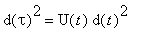 gives
gives
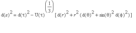
This coincides with the Robertson-Walker interval with zero spacetime curvature . Such constraint is the consequence of the additional field equation on the background metrics. So, the first main consequence of RTG for cosmology:
Space-time of universe is open and flat .
It is necessary to make an important addition to our previous consideration. The field equations in quastion have to be supplemented by the causality principle : since the background spacetime has ontological status, the causality cone of the effective Riemannian spacetime has to lie inside the causality cone of the background Minkowski spacetime ( A.A. Logunov, M.A.Mestvirishvili, "The causality principle in the field theory of gravitation"). As a result:
![mu[m,n]*u^m*u^n = 0](images/rtg1191.gif) ,
,
![g[m,n]*U^m*U^n](images/rtg1192.gif) =<0,
=<0,
where
![]() is the arbitrary isotropic vector. Hence from the expression for the interval
is the arbitrary isotropic vector. Hence from the expression for the interval
 we have
 =
=
 =<0.
=<0.
So, we have to select only the solutions permiting the expansion of the universe up to some maximal radius (in the case of the nonzero mass of graviton, see below).
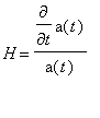
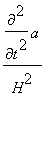
Now we can write the evolutional cosmological equations for such flat universe.
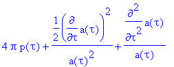
>
subs({C[1]=0,t=tau},eq12):# from eq12 for C[1]=0
op(1,lhs(%)) = - U(tau)*op(2,lhs(%)) ;# d(t)=d(tau)/sqrt(U)
print(`First cosmological equation:`);
fun[13] := expand( subs(U(tau)=a(tau)^6,%)/3 );# U(tau)^(1/3) = a(tau)^2, a(tau) is the scaling factor
![]()
![fun[13] := 8/3*pi*rho(tau) = diff(a(tau),tau)^2/(a(...](images/rtg1199.gif)
>
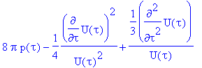
subs(C[2]=0,eq14);# eq14
8*Pi*p(tau) + sqrt(U(tau))*diff( sqrt(U(tau))*diff(U(tau),tau), tau)/U(tau)^2/3 - 5*(sqrt(U(tau))*diff(U(tau),tau))^2/U(tau)^3/12:# d(t)=d(tau)/sqrt(U)
expand(%);
expand( subs(U(tau)=a(tau)^6,%)/2 );
subs(diff(a(tau),tau)^2/(a(tau)^2)=lhs(fun[13]),%) = 0;
>
# Hence
print(`Second cosmological equation:`);
fun[14] := diff(a(tau),`$`(tau,2))/a(tau) = -4*pi/3*(3*p(tau)+rho(tau));
![]()
![fun[14] := diff(a(tau),`$`(tau,2))/a(tau) = -4/3*pi...](images/rtg1205.gif)
These equations are equal to the basic equations of GR in a globally flat space-time.
Massive gravitational field
The field equations in quastion can be generalized on the case of nonzero mass of graviton m . In this case the first equation is:
![R^mn+(1/2)(m^2*(g^mn-g^mk*g^np*mu[pk])) = -8*pi*(T^...](images/rtg1206.gif) ,
,
or in the mixed components
![R[n]^m-delta[n]^m*R/2-m^2*(delta[n]^m+g^mk*mu[kn]-d...](images/rtg1207.gif) .
.
Second field equation on the background keeps its form. Note, that the dimensional coefficients are to be
![]() -->
-->
 and
and
![]() -->
-->
 (
(
![]() is the gravitational constant).
is the gravitational constant).
The equations, which were obtained from
![]() [;]= 0, keep their form and we will consider the previously obtained interval for Riemannian spacetime.
[;]= 0, keep their form and we will consider the previously obtained interval for Riemannian spacetime.
>
coord := [t, r, theta, phi]:
g_compts := array(symmetric,sparse,1..4,1..4):
g_compts[1,1] := U(t):#dtau^2
g_compts[2,2] := -alpha*U(t)^(1/3):#dr^2; alpha is some constant, which can be used for the normalization of the scale factor
g_compts[3,3]:= -alpha*U(t)^(1/3)*r^2:#dtheta^2
g_compts[4,4]:=-alpha*U(t)^(1/3)*r^2*sin(theta)^2:#dphi^2
g := create([-1,-1], eval(g_compts));# covariant components of metric
ginv := invert( g, 'detg' ):
g_scal := det(get_compts(g));# scalar of metric tensor
![g := TABLE([index_char = [-1, -1], compts = matrix(...](images/rtg1214.gif)
![]()
>
mu_compts := array(symmetric,sparse,1..4,1..4):
mu_compts[1,1] := 1:#dtau^2
mu_compts[2,2] := -1:#chi^2
mu_compts[3,3]:= -r^2:#dtheta^2
mu_compts[4,4]:= -r^2*sin(theta)^2:#dphi^2
mu := create([-1,-1], eval(mu_compts));# covariant components of mu
muinv := invert( mu, 'detg' ):
![mu := TABLE([index_char = [-1, -1], compts = matrix...](images/rtg1216.gif)
Now let's write the field equation.
>
D1g := d1metric ( g, coord ):
D2g := d2metric ( D1g, coord ):
Cf1 := Christoffel1 ( D1g ):
RMN := Riemann( ginv, D2g, Cf1 ):
RICCI := Ricci( ginv, RMN ):# Ricci tensor
RS := Ricciscalar( ginv, RICCI ):# Ricci scalar
Estn := raise(ginv, Einstein( g, RICCI, RS ), 2 );# Einstein's tensor with mixed indexes
![]()
![]()
![Estn := TABLE([index_char = [-1, 1], compts = matri...](images/rtg1219.gif)
![]()
>
K_compts := array(symmetric,sparse,1..4,1..4):
K_compts[1,1] := 1:
K_compts[2,2] := 1:
K_compts[3,3]:= 1:
K_compts[4,4]:= 1:
K := create([-1,1], eval(K_compts)):# Kronecker symbol
Z := prod(ginv,mu):
term2 := contract(Z,[2,3]):# second term in brackets (field equation)
ZZ := contract(Z,[2,4]):
prod(K,contract(ZZ,[1,2])):
term3 := prod(table([index_char = [], compts = -1/2]),%):# third term in brackets
Lgv_compts := array(symmetric,sparse,1..4,1..4);
Lgv_compts[1,1] := simplify( get_compts(Estn)[1,1] - ( m^2/2 )*( get_compts(K)[1,1] + get_compts(term2)[1,1] + get_compts(term3)[1,1] ) ):
Lgv_compts[2,2] := simplify( get_compts(Estn)[2,2] - ( m^2/2 )*( get_compts(K)[2,2] + get_compts(term2)[2,2] + get_compts(term3)[2,2] ) ):
Lgv_compts[3,3] := simplify( get_compts(Estn)[3,3] - ( m^2/2 )*( get_compts(K)[3,3] + get_compts(term2)[3,3] + get_compts(term3)[3,3] ) ):
Lgv_compts[4,4] := simplify( get_compts(Estn)[4,4] - ( m^2/2 )*( get_compts(K)[4,4] + get_compts(term2)[4,4] + get_compts(term3)[4,4] ) ):
Lgv := act(expand,create([-1,1], eval(Lgv_compts)));# left-hand side of "massive" field equation
![]()
![Lgv := TABLE([index_char = [-1, 1], compts = matrix...](images/rtg1222.gif)
Hence the first modified field equation is:
>
subs( t=tau,get_compts(Lgv)[1,1] = -8*pi*get_compts(TT)[1,1] ):
subs(diff(U(tau),tau)=sqrt(U(tau))*diff(U(tau),tau),%):
expand( subs(U(tau)=a(tau)^6,%)/3 );# we used diff(U(t),t) = sqrt(U(tau))*diff(U(tau),tau) and U(tau) = alpha^3*a(tau)^6
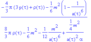
So, we have
>
print(`First Logunov's equation:`);
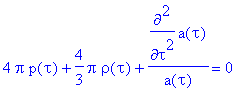
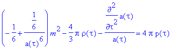
L[1] := diff(a(tau),tau)^2/a(tau)^2 = 8*pi/3*rho(tau) - (1/6)*m^2-1/12*m^2/a(tau)^6+1/4*m^2/(a(tau)^2*alpha);
![]()
![L[1] := diff(a(tau),tau)^2/(a(tau)^2) = 8/3*pi*rho(...](images/rtg1225.gif)
For the second equation we have
> subs( t=tau,get_compts(Lgv)[2,2] = -8*pi*get_compts(TT)[2,2] );
From this
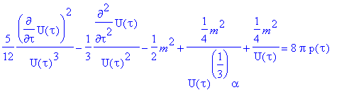
>
-sqrt(U(tau))*diff( sqrt(U(tau))*diff(U(tau),tau), tau)/U(tau)^2/3 + 5*(sqrt(U(tau))*diff(U(tau),tau))^2/U(tau)^3/12 - 1/2*m^2 + 1/4*m^2/(U(tau)^(1/3))/alpha + 1/4*m^2/U(tau) = 8*pi*p(tau):# d(t)=d(tau)/sqrt(U)
expand( subs(U(tau)=a(tau)^6,%) );# we used first equation
subs(diff(a(tau),tau)^2/(a(tau)^2)=rhs(L[1]),%):
simplify( %/2,radical,symbolic ):
collect( expand(%),m^2 );
>
print(`Second Logunov's equation:`);
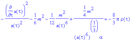
L[2] := diff(a(tau),`$`(tau,2))/a(tau) = -4*pi/3*(rho(tau) + 3*p(tau)) - m^2/6*(1-1/a(tau)^6);
![]()
![L[2] := diff(a(tau),`$`(tau,2))/a(tau) = -4/3*pi*(3...](images/rtg1230.gif)
Cosmological scenarios
Now we will investigate the properties of the system
![]() ,
,
![]() . As the generalization of the results, which were obtained by A.A. Logunov and co-authors, we consider the contribution of the exotic matter (quintessence, X-matter), which can contribute like the cosmological constant [as a survey, see
S. M. Carroll, The cosmological constant]. As the equation of state we choose for the matter (including relativistic forms but without gravitons) the following expression:
. As the generalization of the results, which were obtained by A.A. Logunov and co-authors, we consider the contribution of the exotic matter (quintessence, X-matter), which can contribute like the cosmological constant [as a survey, see
S. M. Carroll, The cosmological constant]. As the equation of state we choose for the matter (including relativistic forms but without gravitons) the following expression:
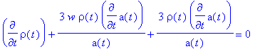
![]() . Then from the covariant conservation law
. Then from the covariant conservation law
![]() [;
n
]= 0 we have:
[;
n
]= 0 we have:
>
d1g:= d1metric(g, coord):
Cf1:= Christoffel1 ( d1g ):
Cf2:= Christoffel2 ( ginv, Cf1 ):
Z := cov_diff( TT, coord, Cf2 ):
act( subs,[U(t)=a(t)^6,p(t)=w*rho(t)],contract(Z,[2,3]) ):
act(expand,%):
get_compts(%)[1] = 0;
This is 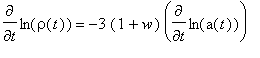 , or
, or ![]() ~
~ 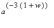 . The simplest situations are:
|
w
|
3(1+ w
)
|
|
|
hard matter
|
1
|
6
|
|
dust
|
0
|
3
|
|
radiation
|
1/3
|
4
|
|
vacuum
|
-1
|
0
|
It should be noted, that the behavior of gravitons in the first Logunov equation corresponds to the hard matter for
a-->
0 and to the vacuum for
a-->
![]() (note also sign "-" for contribution of gravitons).
(note also sign "-" for contribution of gravitons).
Let's use the next parametrization:
 (Hubble function),
![rho[c] = 3*H[0]^2/(8*pi)](images/rtg1241.gif) (critical density,
(critical density,
![]() is the Hubble constant),
is the Hubble constant),
![Omega[m] = 8*pi*rho[m]/(3*H[0]^2)](images/rtg1243.gif) (
(
![]() is the matter density),
is the matter density),
![Omega[r] = 8*pi*rho[r]/(3*H[0]^2)](images/rtg1245.gif) (
(
![]() is the radiation density),
is the radiation density),
![Omega[X] = 8*pi*rho[X]/(3*H[0]^2)](images/rtg1247.gif) (
(
![]() is the density of quintessence),
is the density of quintessence),
![Omega[g] = m^2/(6*H[0]^2)](images/rtg1249.gif) . Tacking into account the causality principle we have for the parameter
. Tacking into account the causality principle we have for the parameter
![]() , where
, where
![]() is the maximal scaling factor.
is the maximal scaling factor.
We will use the modern observational data for cosmological parameters (see L.M. Krauss, Space, time, and matter: cosmological parameters 2001 and D. H. Lyth, Introduction to cosmology):
![]() = 68+/-6
= 68+/-6
 ,
,
![]() = 1.1+/-0.12 (curvature parameter, which is equal precisely to zero in RTG),
= 1.1+/-0.12 (curvature parameter, which is equal precisely to zero in RTG),
![]() = 0.35+/-0.1,
= 0.35+/-0.1,
![]() = 0.65+/-0.15,
= 0.65+/-0.15,
![]() ~ 9.1*
~ 9.1*
 (with the possible contribution of relativistic neutrino,
![]() = 68
= 68
 ),
),
the age of oldest globular clusters is 12.7+/-3 Gyr,
the equation of state of the dominant energy w </= -0.6.
We will vary these parameters within marked boundaries. The main varied parameter will be the mass of graviton. As
w
we will choose the values in the limits of the so-called weak energy condition
![]() >/= 0 and the strong energy condition
>/= 0 and the strong energy condition
![]() >/= 0.
>/= 0.
From
![]() we have the expression for the maximal scaling factor:
we have the expression for the maximal scaling factor:
> subs( {alpha=a[max]^4,a(tau)=a[max]},rhs( L[1] ) ) = 0;
![8/3*pi*rho(tau)-1/6*m^2+1/6*m^2/(a[max]^6) = 0](images/rtg1264.gif)
So
> rho[min] = expand( solve(%,rho(tau)) );
![rho[min] = 1/16*m^2/pi-1/16*m^2/(pi*a[max]^6)](images/rtg1265.gif)
If the turning point is far from the present era, then we can suppose the strong domination of the X-matter density in
![]() . Let's
w
=-1+
. Let's
w
=-1+
![]() (
(
![]() is some positive value). Then
is some positive value). Then
>
Omega[X]*a[max]^(-3*delta) = Omega[g];
fun[15] := solve(%,Omega[g]);
![]()
![]()
> plot([log10( subs({Omega[X]=0.65,delta=0.01,a[max]=10^x},fun[15]) ), log10( subs({Omega[X]=0.65,delta=1/3,a[max]=10^x},fun[15]) ), log10( subs({Omega[X]=0.65,delta=2/3,a[max]=10^x},fun[15]) )],x=0..20,axes=boxed,color=[red,green,blue], title=`Logarithm of Omega[g] vs logarithm of a[max], Omega[x]=0.65`);
![[Maple Plot]](images/rtg1271.gif)
It is obviously, that the
![]() parameter can not be too small, that gives the exaggerated estimation for the graviton mass. Indeed, the repulsion of the vacuum is almost compensated by its attraction due to contribution of the graviton's rest mass. As a result,
parameter can not be too small, that gives the exaggerated estimation for the graviton mass. Indeed, the repulsion of the vacuum is almost compensated by its attraction due to contribution of the graviton's rest mass. As a result,
![]() is close to
is close to
![]() .
.
Estimation of the mass of graviton gives:
>
kappa := 1.86e-27:# gravitational constant [cm/g]
ff := subs({c=3e10,hh=1.054e-27},1/(2*kappa)*(m*c/hh)^2):#hh=h/2/Pi is the Plank constant in [erg*sec]
Omega[g] = subs( rho[g]=ff, subs( rho[c]=1.88e-29*h^2,rho[g]/rho[c] ) ):# rho[c] is the critical density
plot(log10(evalf(subs(h=0.68,m=10^(x),rhs(%)))),x=-75..-65,axes=boxed, title=`Logarithm of Omega[g] vs logarithm of m (in [g], H[0]=0.68)`);
![[Maple Plot]](images/rtg1275.gif)
From the equation
![]() we can obtain the equation for the Hubble function:
we can obtain the equation for the Hubble function:
> basic_1 := H(tau)^2 = H[0]^2*(Omega[r]/(a(tau)^4)+Omega[m]/(a(tau)^3)+Omega[X]/(a(tau)^(3+3*w))-Omega[g]*(1+1/2/(a(tau)^6)-3/2*1/(a(tau)^2*a[max]^4)));
![basic_1 := H(tau)^2 = H[0]^2*(Omega[r]/(a(tau)^4)+O...](images/rtg1277.gif)
At the present era (the cosmic sum rule):
> expand( subs({H(tau)=H[0],a(tau)=1},basic_1)/H[0]^2 );
![1 = Omega[r]+Omega[m]+Omega[X]-3/2*Omega[g]+3/2*Ome...](images/rtg1278.gif)
One can see, that the massive gravitons contribute to the sum rule as a
negative
term. This demands
![]() > 1 (
> 1 (
![]() ~
~
![]() for the large
for the large
![]() ). The modern data give for
). The modern data give for
![]() =1.11+/-0.07 > 1, but we do not rest one's hopes upon the possibilities to reveal the graviton contribution in such measurements (A.H.Jaffe et al. "Cosmology from MAXIMA-1, BOOMERANG, and COBE DMR Cosmic Mocrowave Background Observations", Phys. Rev. Letts.,
86
, 3475 (2001)).
=1.11+/-0.07 > 1, but we do not rest one's hopes upon the possibilities to reveal the graviton contribution in such measurements (A.H.Jaffe et al. "Cosmology from MAXIMA-1, BOOMERANG, and COBE DMR Cosmic Mocrowave Background Observations", Phys. Rev. Letts.,
86
, 3475 (2001)).
Now let's consider the acceleration parameter
 , which is positive at the present era.
> rhs( L[2] )/rhs( L[1] );# acceleration parameter
> fun[17] := -( Omega[m]/2-Omega[X]+3*delta*Omega[X]/2 )/( Omega[m]+Omega[X]-Omega[g]*(1+1/2) );# we used a[max]>>1 and omited the radiation term
![fun[17] := -(1/2*Omega[m]-Omega[X]+3/2*delta*Omega[...](images/rtg1286.gif)
> q = fun[17];
![q = -(1/2*Omega[m]-Omega[X]+3/2*delta*Omega[X])/(Om...](images/rtg1287.gif)
If
![]() >>1 and
>>1 and
![]() <<1, the latter does not contribute essentially into acceleration parameter at the present era. This allows to obtain the estimation for the
<<1, the latter does not contribute essentially into acceleration parameter at the present era. This allows to obtain the estimation for the
![]() parameter:
parameter:
> ff := expand( solve(subs(Omega[g]=0,%),delta) );
![ff := -2/3*q*Omega[m]/Omega[X]-2/3*q-1/3*Omega[m]/O...](images/rtg1291.gif)
>
print(`delta parameter:`);
evalf( subs({Omega[m]=0.44,Omega[X]=0.66,q=0.16},ff) );
evalf( subs({Omega[m]=0.3,Omega[X]=0.76,q=0.5},ff) );
evalf( subs({Omega[m]=0.37,Omega[X]=0.71,q=0.33},ff) );
![]()
![]()
![]()
![]()
> plot([log10( subs({Omega[X]=0.66,delta=0.27,a[max]=10^x},fun[15]) ), log10( subs({Omega[X]=0.76,delta=0.07,a[max]=10^x},fun[15]) ), log10( subs({Omega[X]=0.71,delta=0.37,a[max]=10^x},fun[15]) )],x=0..60,axes=boxed,color=blue, title=`Upper limits of Omega[g] vs logarithm of a[max] for the different delta`);
![[Maple Plot]](images/rtg1296.gif)
And, at last, the estimation of the minimal scaling factor, which has to be smaller than the radius of the universe at the end of the radiation dominated era:
> fun[18] := collect( expand(numer( simplify( rhs(basic_1)/H[0]^2 ) ) )/a[max]^4,a );
![fun[18] := -2*Omega[g]*a(tau)^6+3*Omega[g]*a(tau)^4...](images/rtg1297.gif)
or for
w
~ -1,
![]() >>1:
>>1:
> fun[19] := solve(2*Omega[r]*a(tau)^2-Omega[g] = 0, a(tau));
![fun[19] := 1/2*sqrt(2)*sqrt(Omega[r]*Omega[g])/Omeg...](images/rtg1299.gif)
> plot([subs({Omega[r]=9.1*10^(-5),Omega[g]=10^x},log10(abs(fun[19][1]))),-4],x=0..-30,axes=boxed,title=`logarithm of the minimal scaling factor vs logarithm of Omega[g]`);#horisontal line corresponds to scaling factor at the end of the radiation dominating era
![[Maple Plot]](images/rtg1300.gif)
As a result, we have:
> plot([log10( subs({Omega[X]=0.66,delta=0.27,a[max]=10^x},fun[15]) ), log10( subs({Omega[X]=0.76,delta=0.07,a[max]=10^x},fun[15]) ), log10( subs({Omega[X]=0.71,delta=0.37,a[max]=10^x},fun[15]) ), -11.7],x=0..60,axes=boxed,color=blue, title=`Upper limits of Omega[g] vs logarithm of a[max]`);
![[Maple Plot]](images/rtg1301.gif)
From
![]() we have the expression for the turning points of the accelerated (decelerated) expansion:
we have the expression for the turning points of the accelerated (decelerated) expansion:
> fun[20] := (Omega[m]*a^3+2*Omega[r]*a^2+(-2+delta)*Omega[X]*a^(6-3*delta)) + 2*Omega[g]*(a^6-1);
![]()
> sol := solve(%=0,Omega[g]);
![sol := -1/2*(Omega[m]*a^3+2*Omega[r]*a^2-2*Omega[X]...](images/rtg1304.gif)
The universe evolution has the complicated loitering character:
acceleration - deceleration - acceleration - deceleration - recollapse
. The
![]() parameters providing the era of second deceleration are shown in the next picture (region lying on the right of the curve, the era of the deceleration stops near from
a
=0.7
):
parameters providing the era of second deceleration are shown in the next picture (region lying on the right of the curve, the era of the deceleration stops near from
a
=0.7
):
> plot(subs({Omega[m]=0.44,Omega[X]=0.66,Omega[r]=9.1*10^(-5),delta=0.27,a=10^x},log10(sol)),x=-10..-0.16,axes=boxed,title=`Upper limit of log10(Omega[g]) vs logarithm of a`);
![[Maple Plot]](images/rtg1306.gif)
>
Conclusion
The introducing of the
![]() -term in the Lagrangian of RTG requires
-term in the Lagrangian of RTG requires
![]() =
=
 , which contributes to the deceleration of the universe's expansion. However, the modern observations suggest the accelerated expansion at the present epoch. We showed that this problem can be overcomed by the introducing of the X-matter with the equation of the state, which is close to the extreme weak energy condition
![]() . As a result, the class of the cosmological models in framework of RTG can be extended and there is the cosmological scenario, which is consistent with observational data. We demonstrated, that in the case of
m
<
. As a result, the class of the cosmological models in framework of RTG can be extended and there is the cosmological scenario, which is consistent with observational data. We demonstrated, that in the case of
m
<
 g
and
w
=0.73 - 0.93 the minimal size of the universe, its age and the acceleration at the present epoch do not contradict to the models considered in the framework of GR. The evolution has the complicated loitering character with the alternation of the acceleration and the deceleration.
g
and
w
=0.73 - 0.93 the minimal size of the universe, its age and the acceleration at the present epoch do not contradict to the models considered in the framework of GR. The evolution has the complicated loitering character with the alternation of the acceleration and the deceleration.
2002�Kalashnikov