Velocity Fields of Vibrational Modes of an Elastic Sphere Last updated: January 21, 2008
Velocity Fields of Vibrational Modes of an Elastic Sphere

Graphical illustrations of the velocity fields of exact vibrational modes of an elastic sphere are presented.

   The classic problem of the vibrational modes of an isotropic continuum elastic sphere has been extensively studied [Lamb 1882] [Love 1944] [Auld 1973] [Nishiguchi and Sakuma 1981] [Bastrukov 1994] [Graff 1994] [Bastrukov et al. 1998] [Hanyk et al. 1998 pdf ::] [Ye 2000 pdf], and an accurate list of the exact frequencies has recently been reported [Murray 2002a]. Molecular dynamical simulations of a Lennard Jones like crystalline solid [Murray 2002b] provide numerical evidence to support the correctness of the exact continuum analysis.
   Consider a freely suspended isotropic elastic sphere not subject to body forces. The sphere has radius R, uniform density ρ, shear modulus μ and Poisson ratio ν. These parameters fully describe the problem. If the sphere is disturbed, it will begin to vibrate. A given eigenfunction has frequency ω (in radians per second). The speed of transverse waves (shear waves) is

Cs = sqrt(μ/ρ)

   It is convenient to express normal mode frequencies in terms of the dimensionless variable

η = ω R/Cs

   The displacement field u(x,y,z,t) in the sphere must necessarily be the sum of the gradient of a scalar field and the curl of a divergence free vector field. In past work [for details see Ye 2000 pdf file] the "spheroidal" modes (also known as Rayleigh waves) have a displacement field of the form
u(r,θ,φ,t) exp(-i η Cs t / R ) = An grad [ j(l, kl r ) P(l,cos(θ)) ]
+ Bn curl curl [ r j(l, ks r ) P(l,cos(θ)) ]
while the "torsional" modes (also known as Love waves and called "toroidal" modes in seismology) are of the form
u(r,θ,φ,t) exp(-i η Cs t / R ) = Cn curl [ r j(l, ks r ) P(l,cos(θ)) ]
   Here j(l,x) are spherical Bessel functions of the first kind and P(l,x) are the Legendre polynomials. r is the position vector.    The torsional modes also correspond to choosing the displacement field, (given in spherical coordinates by (ur,uθ,uφ) ) to have the form:

ur = 0
uθ = 0
uφ(r,θ,φ) = - j(l,ks r) d/dθ ( P(l,cos(θ) )

where x = r sin(θ) cos(φ), y = r sin(θ) sin(φ) and z = r cos(θ). The wavevector ks = η / Cs, where the dimensionless frequency η takes on an eigenvalue for each mode.
   The lowest frequency torsional mode (excepting the zero frequency n=1 mode which corresponds to rigid rotation) is for n=2 with η=2.502. In this case, j(2,x) is approximately x2, and since P(2,x) = (3 x2 - 1 )/2 consequently d/dθ P(2,cos(θ) ) = - 3 cos(θ) sin(θ). In Cartesian coordinates the (approximate) displacement field is

ux = -z y cos(ω t)
uy =  z x cos(ω t)
uz = 0

   The top half of the sphere (z>0) thus rotates clockwise while the bottom half of the sphere rotates counterclockwise. The plane z=0 remains stationary. This motion is reminiscent of the thrashing motion that a dog makes in order to shake water off its fur. The head of the dog rotates in a direction opposite to the rotation of the rest of its body. This mode could be called a "wet dog" mode.

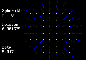
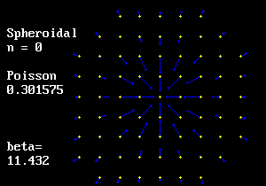
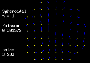
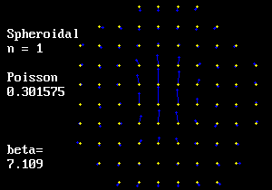
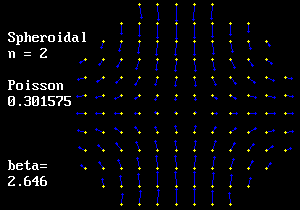
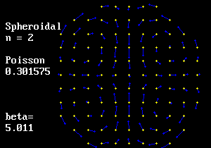
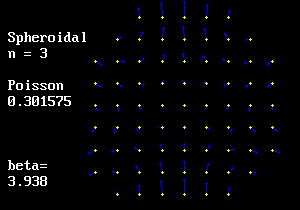
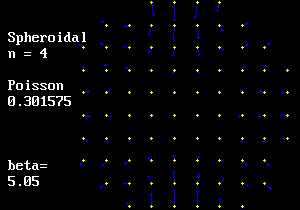
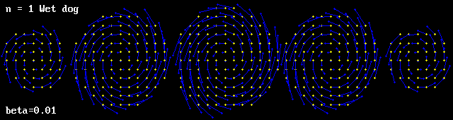
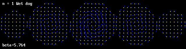
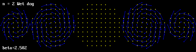
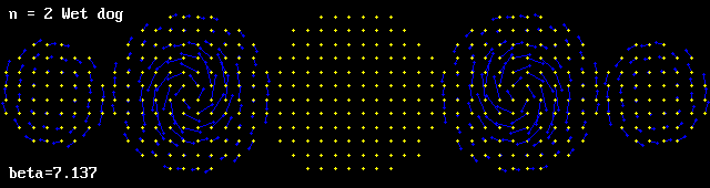
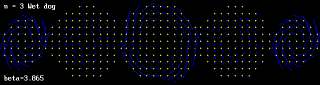
Figure 1.The velocity fields of the spheroidal modes of an elastic sphere are shown. A slice through the center of the sphere is shown. Blue arrows show the velocity at representative points. The z-axis points towards the top of the page. (Jul 8 02 velfie2b.cpp zsph0.gif...)
 

Figure 2. The velocity fields of the torsional modes of an elastic sphere are shown. The sphere is illustrated in five slices. The slices are at z = {0.8R, 0.4R, 0, -0.4R, -0.8R} where R is the radius of the sphere. The topmost (z=0.8R) slice is at the left. The bottom slice is at the right. Blue arrows show velocity in the plane of the page. (velfield.cpp, picsph0.gif, picsph0b.gif, picsph1.gif ...)
 

References:

H. Lamb, Proc. London Math. Soc. 13, 187 (1882).)
A. E. H. Love, A Treatise on the Mathematical Theory of Elasticity, (Dover, New York, 1944).
B. A. Auld, Acoustic Fields and Waves in Solids, (John Wiley & Sons, New York, 1973).
N. Nishiguchi and T. Sakuma, Sol. Stat. Comm. 38, 1073 (1981).
Sergey I Bastrukov, Phys. Rev. E 49, 3166 (1994).
F. K. Graff, Wave Motion in Elastic Solid, (Ohio University Press, Ohio, 1994).
Bastrukov et al., Physica A 250, 435 (1998).
Zhen Ye, "On the Low Frequency Elastic Response of a Spherical Particle" Chinese Journal of Physics Vol. 38, pages 103-110, (2000). pdf
L. Hanyk, C. Matyska and D. A. Yuen "Initial value approach for viscoelastic responses of the earth's mantle" 1998. (pdf ::)
Daniel B. Murray, "Molecular Dynamics Simulation of an Elastic Material" 2002 (link to article)
Daniel B. Murray, "Vibrational Frequencies of an Elastic Sphere" 2002 (link to article)
Daniel B. Murray, "Molecular Dynamical Estimates of Vibrational Frequencies of a Crystalline Sphere" 2002 (link to article)
Daniel B. Murray, "Toroidal Vibrational Modes of an Elastic Sphere" 2002 (link to article)

Daniel Murray
Associate Professor
Math, Stats & Physics Unit
University of British Columbia - Okanagan
Kelowna, BC, Canada
daniel "dot" murray "at" ubc "dot" ca

For a list of related articles click on the link.

Hosted by www.Geocities.ws

1