Tensors – The
Analytic View
Back
to Physics World
Back to Geometrical Math for GR
Position
vector: Let DX
= (Dx,
Dy,
Dz)
represent a vector displacement (i.e. an arrow) between two points, one point of
which is located at the tail of the arrow and the other point located at the tip
of the arrow. Now designate the point where the tail of the arrow lies as the origin
of the coordinate system. The tip of the arrow is at the location of
interest, e.g. the location of a particle.
Then the displacement vector is referred to as the position vector
and denoted here as X = (x, y, z), a point, P,
in a flat manifold.
The transformation from one set of Cartesian coordinates to another set under an
orthogonal transformation, is a transformation
where, as an example, a new coordinate system is obtained from an old system
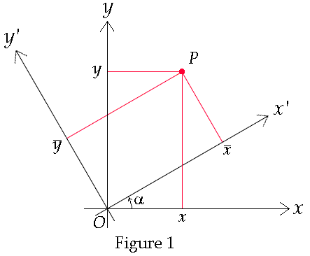
through a rotation of the axes of the original system, as shown in Figure 1
below. In that figure the xy-plane is rotated about the z-axis.
We
can represent this mathematically as
![]()
where
R represents the rotation matrix which represents an orthogonal
transformation. In this case it is a function of a,
i.e. R = R (a).
Some quantities remain unchanged by such a transformation. For example: consider
a sheet of steel lying in the xy plane and let T(P) represent
the temperature of the plate at a given point P on the surface of this
manifold. If the surface temperature is non-uniform then T will vary over
the surface and thus T will be a function of position P. This is
expressed as T = T(P) or as T = T(x, y).
Since the temperature is independent of the particular coordinate system then we
have
![]()
Such a
quantity, i.e. a number that does not depend on a particular coordinate system,
is called a scalar. This can obviously be extended to three dimensions by
applying additional rotations about different axes. This relation motivates the
following definition
Definition:
Any one-component quantity F
defined on a manifold whose numerical value remains unchanged under an
orthogonal transformation is called an affine scalar (aka scalar)
or an affine invariant (aka invariant). I.e. If
![]()
then
F
is a scalar. The notation F’
means that the value of the value of the function at the point is the same but
that the function may take on a new form, i.e. have a different functional
dependence on the new variables. A
scalar is also referred to as a tensor of rank zero.
Not all
geometric quantities are scalars. Consider the components of the position vector
when it is expressed in Cartesian coordinates. The components transform under an
orthogonal transformation as
![]()
This
equation may be placed in matrix form as
![]()
The
components of A are constant in time. Let us some examples from classical
mechanics. Let xi
represent
the position of a particle with respect to a Cartesian coordinate system.
Differentiating Eq. (3) with respect to time gives the linear velocity vi
=
dxi
/dt.
I.e.
If Eq.
(6) is multiplied by the particle's mass then the result will be the particle's
linear mechanical momentum. Therefore
the momentum transforms as
Differentiating
once more with respect to time will then give the transformation relation for
the components of the force acting on the particle, i.e. Fi
=
dPi
/dt.
The expression for force in Cartesian coordinates is given by
![]()
In what follows Einstein's
summation convention will be employed
Einstein's
Summation Convention:
If an index appears twice in a term, once as a superscript and once as a
subscript, then summation is implied over the range that the indices are allowed
to take on.
Thus,
using the summation convention for Eqs. (4) - (8) become
![]()
This
motivates the following definition
Definition:
Any set of n quantities {A1,
A2,
... , An}
which transform under an orthogonal coordinate transformation as
![]()
is
called an affine vector (or simply vector) or an affine tensor
of rank one (or simply a tensor of rank one).
If n = 3
the affine vector is known as a Cartesian vector. The components of a vector change from one coordinate system
to another and are therefore not invariant. A number that is not invariant is
called covariant. [1] However arc length is remains unchanged and
therefore is invariant. Consider now the infinitesimal arc-length of a portion
of a curve, C, as shown in Figure 2
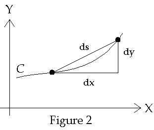
The arc
length, ds, between two points on the curve is given in Cartesian
coordinates, approximately, by
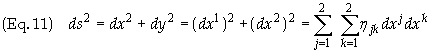
where hjk = djk is the Kronecker Delta defined as; djk = 1 when j = k and 0 otherwise. Using the summation convention, applied to both indices, reduces Eq. (6) to
![]()
which
looks much simpler! Generalizing the arc length to three dimensions gives
![]()
The
range of values for both j and k are now 1, 2, 3 rather than 1
and 2. This information is known from the particular application. Arc
length, ds, may also be expressed in coordinate systems other than
Cartesian. For example we can use polar coordinates to express the arc length.
Consider the coordinate increments dr and df
as shown in Figure 3 below
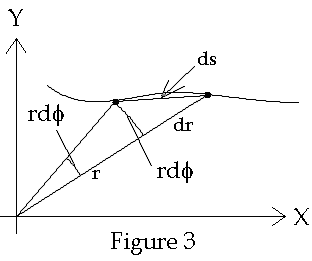
Then the
arc length is given by
![]()
where x1
º
r, x2
º
f,
and g00
= 1, g11
º r2,
and gjk
= 0 otherwise. The infinitesimal arc length, ds, represents the shortest
distance between two closely spaced points on any surface whether that surface
is flat or curved. If the surface is flat and the coordinates are Cartesian then
we will use the symbol of gjk
=
hjk
. The term interval is used as a general term for ds. (Sometimes
it is used to refer to ds2).
It may represent arc length as it has here or it may represent something else,
such as the spacetime interval. The ideas above motivate the following
definition
Definition:
Given a definition of ds in terms of the coordinate differential curvilinear
coordinates dqi,
the equation
![]()
is
called the metric (which means measure). The metric should not be
confused with the metric tensor g whose components in the chosen basis
are gjk
.
Therefore
the metric is a measure of the interval between two closely spaced points. This
metric motivates the definition of a second rank tensor.
Affine
Second Rank Tensor:
Any quantity Ajk that transforms under
orthogonal transformations
![]() as follows
as follows
![]()
is
called an affine tensor of rank two.
An affine tensor of a given rank (number of indices) in R3
is also known as a Cartesian tensor.
Example - Tidal
Force Tensor:
Consider the tidal
force tensor is a Cartesian tensor whose components have the value
![]()
where F
is the Newtonian
gravitational potential, which is a Cartesian scalar. Consider
the orthogonal transformation
![]() . The inverse of this transformation is
. The inverse of this transformation is
![]() . Using the chain rule for partial derivatives
. Using the chain rule for partial derivatives
![]()
Now take the second partial derivative
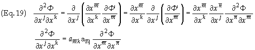
Eq. (19) can be rewritten
by an exchange of variables relating to a orthogonal transformation in the
opposite direction which would yield
![]()
Thus the qualifier tensor
in tidal force tensor is justified.
Contravariant
Vector: Let aa
be an ordered set of n real numbers (i.e. an n-tuple) associated with a
point P(xb)
in Rn. Let xa
= xa(x1,
x2, ... , xn) be an allowable coordinate
transformation. Let
![]() be
associated with P with respect to the coordinate system xb.
If
be
associated with P with respect to the coordinate system xb.
If
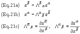
Then the quantities ab are said to be the components of a contravariant vector or contravariant tensor of rank one. Another term for this quantity is simply a general vector. The contravariant transformation property is indicated by a superscript.
The position vector of a
point x = (x1, x2, ... , xn)
(n = dimension of the space) is a function of a set of coordinates xa.
If all but one coordinate fixed and that one coordinate is varied then the point
will trace out a curve. Let ds be the arc distance between two closely
spaced points. If dx is the difference between two closely
spaced points on such a curved then dx will be tangent to the
curve and ds = |dx|. Thus ¶x/¶xa
will be a vector tangent to the curve obtained by varying only xa.
These coordinates will, in general, be arbitrary and they represent mutually
independent variables. They are referred to as curvilinear coordinates
and they uniquely determine a point in the space. The set of N vectors ¶x/¶xa
will allow one to expand any vector in terms of these vectors. Such a set is
said to form a basis. These basis vectors are thus defined as
![]()
The interval ds
(sometimes referring to ds2)
is defined through
![]()
dx can be expanded as
![]()
It is noted here that ds2
can be obtained from the metric as follows
![]()
References:
[1] The usage of the term covariant here is consistent with the usage in The Variational Principles of Mechanics - 4th Ed, by Cornelius Lanczos, Doover Pub. (1970). See pages 20 and 292.