Orthogonal Transformations

Back to Physics World
Back to Geometrical Math for GR

Einstein's Summation Convention

Typically the unit vectors i, j, and k are used in vector analysis in Cartesian coordinates to represent the unit vectors which are parallel to the x, y and z axes, respectively. I.e. any vector A can be represented in terms of these unit vectors as

If we change notation then Einstein's summation convention can be used, i.e.

Einstein's Summation Convention: If an index appears twice in a term, once as a superscript and once as a subscript, then summation is implied over the range that the indices are allowed to take on.

Example: Define the following

The summation convention can now be used to express A 

Similarly we can choose another Cartesian coordinate system, rotated with respect to the first, and thus use another basis to express A, i.e.

Bases

If all vectors in an n-dimensional vector space Rⁿ can be written in terms is the set of vectors V = {v¹, v², .... , v^m} then the set is said to span Rⁿ. The V set is called a spanning set of S. If

implies that l^k = 0 for all k then the vectors in V are said to be linearly independent. It can be shown that the dimension of a linearly independent spanning set has dimension m = n.  If any vector in Rⁿ can be written in terms of a set, V, of linearly independent vectors which spans Rⁿ then that set is called a linearly independent spanning set, or simply a basis, for Rⁿ. It can be shown that the number of basis vectors equals the dimension of the vector space, i.e. m = n. If the magnitude of all the vectors in the basis equals one then that basis is said to be normalized. If the set of vectors are orthogonal, i.e. then they further satisfy the relation e_k·e_j = d^k_j, where d^k_j is the Kronecker delta which has the value 1 when k = j and zero otherwise, then the basis is said to be orthogonal. If the basis is both orthogonal and normalized then the basis is said to be orthonormal.

Note: The basis  {v¹, v², .... , vⁿ}  will be represented simply by writing {vⁿ} unless otherwise noted.

Orthogonal Transformations

For purposes of illustration a 3-dimensional Cartesian coordinate system will be used. However the concepts presented here apply to n dimensions. Let {e_j} and { } be two different orthonormal bases. Since the bases are orthonormal if follows that e_k·e_j = d^k_j and . Any position vector r can be represented as

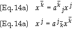
In order to solve for  in terms of x^j take the dot product of each side of Eq. (6) and use the orthogonality conditions and the definition , I.e.

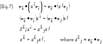
This result represents the transformation . This same procedure can be used to solve for x^k, as follows

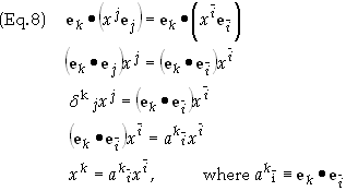
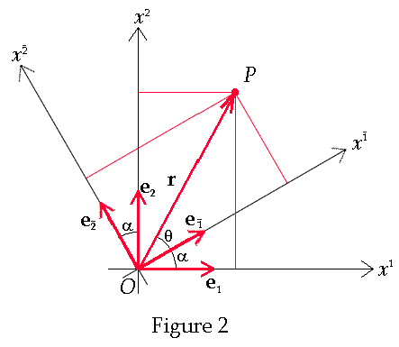
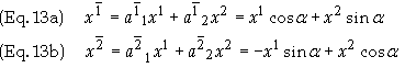
This result represents the transformation .  Example: Consider the passive transformation that results from rotating the xy-axis and representing the components of the position vector in terms of the new axes as shown below

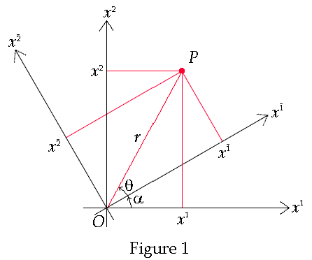
We can find the new coordinates  in terms of the old coordinates (x¹, x²) in two different ways. The first is geometrically and the second using the method described above. Using the geometric method first we start by referring to the diagram and note that

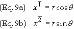
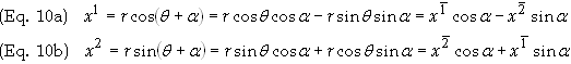
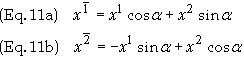
Eq. (10) can readily be solved for  in terms of (x¹, x²) to give

The other method mentioned above requires that we first find the direction cosines , which can be picked off from the Figure 3 below

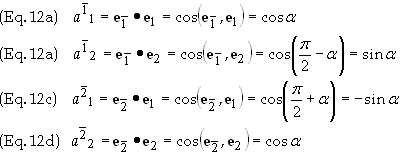
When Eq. (12) is substituted into Eq. (7) the transformation in Eq. (11) readily results.

Recall Eqs. (7) and (8) above, i.e.

which implies

This expression is known as the orthogonality condition. In matrix language Eq. (14a) may be expressed as

Likewise Eq. (14b) may be expressed as

where AT is the transpose of A. The orthogonality condition may now be written as

This implies that AT is the inverse of A, i.e.

Definition of Orthogonal transformation [1]: Any linear transformation that has the property is called an orthogonal transformation and  is known as the orthogonality condition.

References:

[1] Tensors, Differential Forms, and Variational Principles, David Lovelock and Hanno Rund, Dover Pub., pages 19 to 21.

Back to Geometrical Math for GR
Back to Physics World