About Dr. Ernest Ising
What is the Ising model?
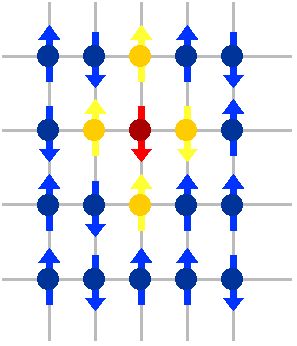
The Ising model can be understood as a bunch of little arrows(spins) arranged on a checkerboard(lattice of atoms), with the constraint that each arrow is pointing either up or down(that is no sideways pointing are allowed).
A Simple Ising Model Universe
In the Ising model, the system considered is an array of N fixed points called lattice sites that form an n-dimensional periodic lattice(n = 1,2,3). The geometrical structure of the lattice may(for example) be cubic or hexagonal. Associated with each lattice site, is a spin variable S(i),(i = 1,...N), which is a number that is either +1 or -1. There are no other variables. If S(i) = +1, then the S(i) site is said to have spin up, and if S(i) = -1, it is said to have spin down. A given set of numbers{S(i)} specifies a configuration of the whole system.
That is:
A State in the Ising model is simply the specification of the spin(up or down) at each of the lattice sites.
The energy of the system in the configuration specified by {S(i)}is usually written as a sum of two terms:
(a) An interaction term for sets of 'nearby' spins on the lattice.
(b) A possible additional interaction term from interaction of the
individual spins with external magnetic field.
In the standard (and simplest form) of the Ising model, the interactions among the little spin vectors are restricted to Nearest Neighbors. That is, in the drawing above:
"The Red Site Only Interacts With The
Four Immediately Adjacent Yellow Sites."
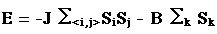
This leads to a fairly simple expression for the energy of any particular state in the Ising model. So the energy of any
particular state is given by:
 .....(1)
where,
S(j) (written with a subscript 'j' in the equation) is the
value of the spin at the j-th site in the lattice, with S =
+1 if the spin is pointing Up and S=-1 if the spin is pointing
Down.
.....(1)
where,
S(j) (written with a subscript 'j' in the equation) is the
value of the spin at the j-th site in the lattice, with S =
+1 if the spin is pointing Up and S=-1 if the spin is pointing
Down.
The < i,j > subscript on the summation symbol indicates
that the spin-spin interaction term, S(i)*S(j) is added up over
all possible nearest neighbor pairs.
The constant J has
dimensions of energy (e.g., it could be specified in something
like ergs) and it measures the strength of the spin-spin
interaction. If J is positive, the energy is lowered when
adjacent spins are aligned.
This is the usual model for
ferromagnetism. If the interaction energy is negative, the
energy is minimized when adjacent spins alternate - a
phenomenon usually called anti-ferromagnetism. The constant B
(again, an energy), indicates an additional interaction of the
individual spins, with some external magnetic field.
From expression(1), we can say that energy is low if:
S(i) and S(j) are parallel.
S(i) is in the direction of magnetic field.
In this case, there are two competing forces:
(1) Thermal energy
(2) Exchange interaction
At high temperatures, (a) is dominant (increasing temperature tries to disalign the spins
and at low temperatures, (b) is dominant.
Assumptions
We assume the following:
Atoms are all fixed at one point(characterized by spin up or down). That is; the position of atoms in lattice is not changing.
Only nearest neighbours interact(for simplification).
So, J(ij) =J if i and j are nearest neighbours
When i and j are not nearest neighbours, J(ij) = 0
What are we looking at in the model?
We look at a particular domain of a ferromagnetic material and study the following:
Thermal properties
(a) Average Energy (< E >)
(b) Average Magnetization (< M >)
(c) Specific Heat (C)
(d) Magnetic Susceptibility ( )
)
Phase transition and Critical phenomenon
We see that in zero magnetic field there is a continuous phase transition (spontaneous magnetization occurs), with a logarithmic singularity in various thermodynamic properties, at the critical point.
The Monte-Carlo Method
History of Monte Carlo Method
MOTIVATION -The problem of summing
The macroscopic quantities may seem to be simply calculated by doing probability sums.
Moreover, the relationship between the number of sites in the "Ising Universe" and number of different states of the system is :
 (two orientations at the first site times two orientations at the second site times .....)
The 2^N(2 raised to the power N) behaviour for number of states is a computational 'disaster'.
For a small 16 X 16
lattice ( 256 total sites ), there are about 10^77 different states in the probability
sum. Being generous, a really really fast computer might be able to evaluate about 10^10
individual terms per second and the entire calculation would be completed in about 10^67
seconds.
In contrast, the age of universe is about 10^20 seconds!
What should be done?
One particularly clever thing to do is to pick out only the 'important' states in the
probability sum.
Consider a system of spins in equilibrium with an external heat source at
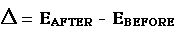
temperature T. The system evolves through a number of independent, random spin flips. An
individual spin flip has an associated change in the overall system energy:
 And according to the standard Boltzmann distribution, the likelihood that this transition occurs, is of the form :
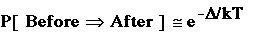 Now, consider a Computer Algorithm which attempts to mimic nature by selecting individual sites within the (simulated) lattice at random.
At the selected site, deciding to flip or not flip the current spin, with the spin-flip
probability given by the Boltzmann probability function.
Now, consider a Computer Algorithm which attempts to mimic nature by selecting individual sites within the (simulated) lattice at random.
At the selected site, deciding to flip or not flip the current spin, with the spin-flip
probability given by the Boltzmann probability function.
After some number of passes through the lattice to change the initial spin assignments,
this procedure generates spin configurations which naturally follow the real probability
function. Physical quantities (such as total magnetization) can then be evaluated by simply
averaging the values of that quantity over the simulated samples.
There are two qualitative reasons, why this is a reasonable procedure for estimating average
quantities for interacting systems:
1. The procedure does not waste a whole lot of time generating or examining improbable
configurations.
2. Rather than exploring "all" configurations--including the enormous numbers of
configurations which are extremely similar in terms of macroscopic quantities--the algorithm
meanders along a modest number of representative paths.
The procedure randomly samples states according to the real underlying probability
distribution. This, in turn, makes it possible to estimate system averages with reasonable
sized simulation samples (eg. a few thousand samples).
The name Monte Carlo refers to the famous Casino in Monaco, and emphasizes the
important role of random decisions within the algorithm.
Metropolis Algorithm (Importance Sampling)
The Ising Model employs the Metropolis algorithm in order to show that the overall energy of
the lattice is converging. The Metropolis algorithm involves flipping a random lattice
point, and determining if the net energy decreases.
If the energy decreases because of
the random flip, then the new state is allowed, and the simulation continues.
If the new
lattice configuration causes the overall energy to increase, then a random number between 0
and 1 is generated.
If the exponential of the temperature and change in energy is less than
this randomly generated number, then the state is allowed, and the simulation continues.
If
this exponential is less than the randomly generated value, the flip is not allowed. In that case the
flipped lattice point is returned to its previous state, a different random lattice point is
chosen and the simulation continues.
Here is the Metropolis Algorithm in step form:
1. Choose an initial configuration of spins.
2. Pick one spin and calculate the energy change dE, if that spin is flipped.
3. If dE < 0, then you flip that spin.
4. If dE > 0, then you flip that spin with a probability 
(NOTE here that, if dE is large, then probability of flipping that spin is small and
vice-versa)
5. Repeat steps 2 to 5 for all spins and many times over, until you get the most probable
state (i.e. the equilibrium state)
The program(in fortran-77)
Simulation Results and Discussion
Study of Phase Transition and critical Phenomenon in the 3D Ising lattice
We studied the phase transitions and critical phenomenon in the three
dimensional Ising model and obtained the following results:
Average energy Vs temperature
Average Magnetization Vs temperature
Specific Heat Vs temperature
Magnetic susceptibility Vs temperature
 Want to know how magnets work? I'll tell u!
Conclusion from the graphs
A characteristic signature of a continuous phase transition is the divergence of specific heat and magnetic susceptibility at the critical point.
The graphs above show that there is continuous phase transition at T=4.52, which matches with results obtained in the past.
Calculating Critical Exponents
Here we shall discuss the method of finding the critical exponents that we have taken into account.
1. Order Parameter critical exponent:
We take values of T, very close to (but below  ), i.e.:in the region where < M > is beginning to be greater than zero till it becomes 0.9 (T for which 0.9 and
  for each T.
Now, we know that order-parameter critical exponent is given by  < M > can be written as:
 Taking ln on both sides:
 A plot between ln< M > and ln tau_beta is a straight line, whose slope gives the order-parameter critical exponent,
2. Susceptibility critical exponent:
We take values of T, close to and find and  at each T.
We know that susceptibility critical exponent is given by
at each T.
We know that susceptibility critical exponent is given by  and can be written as:
 Taking ln on both sides:
 A plot between
  and
and  is a straight line, negative of whose slope gives the susceptibility critical exponent,
3. Specific heat critical exponent:
We take values of T, close to and find  and
and  at each T.
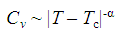
We know that specific heat critical exponent is given by
at each T.
We know that specific heat critical exponent is given by  and can be written as:
 Taking ln on both sides:
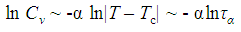 A plot between
  and
and  is a straight line, negative of whose slope gives the specific heat critical exponent,
The Plots for various thermodynamic quantities that show scaling behaviour for T close to are as follows:-
< M > Vs 
Vs 
Vs 
Correctness of the obtained critical exponents:
The values obtained for various critical exponents are universal. Further, these critical exponents nearly satisfy the "Rushbrooke" scaling law, viz:
+ 2 + = 2
|
References
Statistical Mechanics, by Kerson and Huang.
ICTP Lecture notes,by I. Vilfan.
Resource letter: Jan Tobochnik.
Ising Model Application Hrothgar K-12 Project
|
Check:
We have obtained:
= 0.15
= 0.32
= 1.30
=>
+ 2 + = 0.15 + 2(0.32) + 1.30 = 2.09 
Shaista Ahmad
Department of Physics,
Jamia Millia Islamia,
New Delhi 110025, India
E-mail: shaista jamia-physics.net
