C.6 Final Form of the Lorenz Equations

Versão em Português

We now substitute the assumed forms for the streamfunction and the temperature deviation function into Eqs. (C.4-2) and (C.4-5). As we do so, we find that most terms simplify. For example, we have

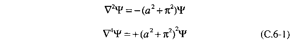
The net result is that some of the complicated expressions that arise from .grad v terms disappear, and we are left with

The only way the previous equation can hold for all values of x and z is for the coefficients of the sine terms to satisfy

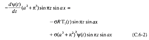
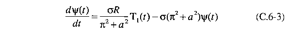
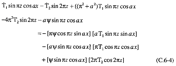
The temperature deviation equation is a bit more complicated. It takes the form

We first collect all those terms which involve sin πz cos ax. We note that the last of these terms in Eq. (C.6-4) is 2aπψT₂ sin πz cos ax cos 2πz. Using standard trigonometric identities, this term can be written as the following combination of sines and cosines: (-1/2 sin πz+1/2sin 3πz) cos ax. The sin 3πz term has a spatial dependence more rapid than allowed by our ansatz; so, we drop that term. We may then equate the coefficients of the terms in Eq. (C.6-4) involving sin πz cos ax to obtain

All the other terms in the temperature deviation equation are multiplied by sin 2πz  factors. Again, equating the coefficients, we find

To arrive at the standard form of the Lorenz equations, we now make a few straightforward change of variables. First, we once again change the time variable by introducing a new variable t´´ = (π² + a²)t'. We then make the following substitutions:

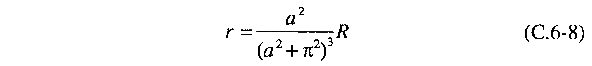
where r is the so-called reduced Rayleigh number:

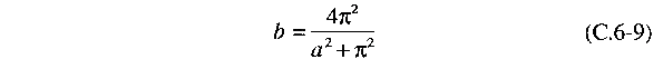
We also introduce a new parameter b defined as

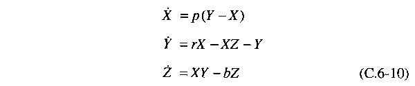
With all these substitutions and with the replacement of σ with p for the Prandtl number, we finally arrive at the standard form of the Lorenz equations:

At this point we should pause to note one important aspect of the relationship between the Lorenz model and the reality of fluid flow. The truncation of the sine-cosine expansion means that the Lorenz model allows for only one spatial mode in the x direction with "wavelength" 2π/a. If the actual fluid motion takes on more complex spatial structure, as it will if the temperature difference between top and bottom plates becomes too large, then the Lorenz equations no longer provide a useful model of the dynamics.

Let us also take note of where nonlinearity enters the Lorenz model. We see from Eq. (C.6-10) that the product terms XZ and XY are the only nonlinear terms. These express a coupling between the fluid motion (represented by X, proportional to the streamfunction) and the temperature deviation (represented by Y and Z, proportional to T₁ and T₂, respectively. The Lorenz model does not inc1ude, because of the choice of spatial mode functions, the usual .grad v nonlinearity from the Navier-Stokes equation.