Arrange the given observations from smallest to largest. That is, the sample is arranged as x(1), x(2), ... x(j), ..., x(n), where x(1) is the smallest observation, x(2) is the second smallest observation, and so on, with x(j) the jth smallest observation and x(n) the largest.
Determine the observed cumulative frequency fraction (j-0.5)/n for each observation, where j is the serial number of the ordered observations.
If probability paper is available, plot x(j) vs (j-0.5/n) on the paper.
If probability paper is not available, determine the standard normal variable zj such that the area from -infinity to zj under the standard normal curve is equal to the cumulative frequency fraction corresponding to each x(j) or in other words, such that
In Excel, you can use the NORMSINV() function to determine the zj s.
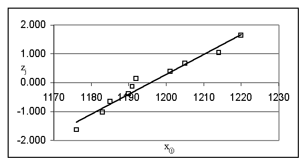
Plot zj vs x(j).
If the distribution is normal, the plotted points will fall approximately along a straight line; otherwise not.
Example:
Question:You are given 10 observations of a variable: 1176, 1191, 1214, 1220, 1205, 1192, 1201, 1190, 1183, and 1185. Construct a normal probability plot for this data.
Answer:
Table
j
x(j)
(j-0.5)/10
zj
1
1176
0.05
-1.645
2
1183
0.15
-1.036
3
1185
0.25
-0.674
4
1190
0.35
-0.385
5
1191
0.45
-0.126
6
1192
0.55
0.126
7
1201
0.65
0.385
8
1205
0.75
0.674
9
1214
0.85
1.036
10
1220
0.95
1.645
Reference:
Montgomery, Douglas C., "Introduction to Statistical Quality Control - Third Edition", John Wiley & Sons Inc., New York, 2001, pp.114-115.