(Excerpted from Draper, Norman R. & Smith, Harry, "Applied Regression Analysis Third Edition", John Wiley & Sons Inc, New York, 1998, pp. 86-89)
We have dealt with the fitting of a straight line model Y = bo + b1X + e to a set of data (Xi, Yi), i = 1, 2, . . . , n. We have also carefully considered a detailed analysis of how well the line fits, and whether or not repeated observations indicated whether or not there was any evidence in the data to indicate that an alternative model should be used. When we have only one predictor variable X and when the postulated model is a straight line, the alternatives we would consider would often be higher-order polynomials in X; for example, the quadratic Y = bo + b1 X + b11 X2 + e, or the cubic, and so on. We now put all this information into a practical perspective by considering the problem of choosing an experimental strategy for the one-predictor-variable case.
Suppose an experimenter wants to collect data on a response variable Y at n selected values of a controllable predictor variable in order to determine an empirical relationship between Y and the predictor variable. We assume that the latter is (at least to a satisfactory approximation) not subject to random error, but that Y is, and that the n values of the predictor are not necessarily all distinct, that is, repeat runs are permitted The experimenter first has to ask, and answer, a number of questions.
1. What range of values of the predictor variable is she currently interested in? This is often difficult to decide. The range must be wide enough to permit useful inference, yet narrow enough to permit representation by as simple a model function as possible. Once the decision is made, the interval can be coded to (-1, 1) without loss of generality. For example, if a temperature range of 140°F <= T <= 200°F is selected, the coding2. What kind of relationship does the experimenter anticipate will hold over the selected range? Is it first order (i.e., straight line), second order (i.e., quadratic), or what? To decide this, she will not only bring to bear her own knowledge but will usually seek the expertise of others as well. To fix ideas, let us assume the experimenter believes the relationship is probably first order but is not absolutely sure.
3. If the relationship tentatively decided upon in (2) is wrong, what alternative does the experimenter expect? For example, if she believes the true model is a straight line, she is most likely to expect that, if she is wrong, the model will be somewhat curved in a quadratic manner. A more remote possibility is that the true model may be cubic. Typically, she will decide that she may be one order too low, if anything. Otherwise, she would probably postulate a higher-order model to begin with.
4. What is the inherent variation in the response? That is, what is V(Y) =s2? The experimenter may have a great deal of experience with similar data and may "know" what s2 is. More typically, she may wish to incorporate repeat runs into the experiments so that s2 can be estimated at the same time as the relationship between Y and X, and also so that the usual assumptions about the constancy of s2 throughout the chosen range of values of the predictor can be checked.
5. How many experimental runs are possible? The experimenter has only limited dollars, staff, facilities, and time. How many runs are justified by the importance of the problem and the costs involved?
6. How many sites (i.e., different X-values) should be chosen? How many repeat runs should be performed at each of the chosen sites?
Let us now continue our discussion in terms of a specific example.
Suppose our experimenter decides that a straight line relationship is most likely over the range -1 <= X <= 1 of her coded predictor, that she most fears a quadratic alternative, that she does not know s2, and that 14 runs are possible. At what values of X (i.e., what sites) should she perform experimental runs, how many where, and with what justification?
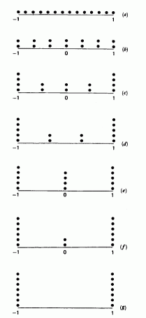
Figure 3.4 shows some of the possibilities. (Each dot represents a run; a pile of dots represents repeated runs.) Let us see how each matches the requirements we have set out.
|
|
| Figure 3.4: Some possible experimental arrangements for obtaining data for fitting a straight line: (a)14 sites, (b) 7 sites, (c) 5 sites, (d) 4 sites, (e) 3 sites, (f) 3 sites, and (g) 2 sites. Which are good, which are bad, in the circumstances described in the text? The sites are equally spaced in cases (a)-(f). |
Each design has 14 degrees of freedom to begin with. Two of these are taken up by the parameter estimates b0 and bl leaving 12 residual degrees of freedom to be allocated between lack of fit and pure error. Lines (1) and (2) of Table 3.1 show how these residual degrees of freedom split up for the various designs. Line (3) gives the value of
SXX-½ = {S(Xi -`X)2}-½ ,
which, by Eq. (1.4.6), is proportional to the standard deviation of bl when a straight line is fitted. Line (4) shows the number of parameters that it is possible to fit to the design data. We can fit a polynomial of order p - 1 (with p parameters including b0 to a design with p sites. A second reason that this is shown is that p is proportional (when n and s2 are fixed) to s2/n, and the latter is the average size of V(Y^(X)) averaged over all the points of the design when the polynomial of order p - 1 is fitted. In other words
n
S V{Y^(Xi)}/n = ps2/n.
i=1
This result is true in general for any linear model. For the straight line case, when p = 2, it can be deduced by replacing the subscript 0 by i in Eq. (3.1.3), summing from i = 1, 2, . . . , n, and dividing by n. For a general proof using matrices see Exercise R in "Exercises for Chapters 5 and 6."
Note that the lack of fit degrees of freedom is equal to the number of distinct X-sites in the data minus the number of parameters in the postulated model. In fact, because our example has two parameters to be estimated, b0 and b1, line(4) minus line(1) equals 2 throughout Table 3.1| TABLE 3.1. Characteristics of Various Strategies Depicted in Figure 3.4 | |||||||
|---|---|---|---|---|---|---|---|
| (a) | (b) | (c) | (d) | (e) | (f) | (g) | |
| (1) Lack of fit df: | 12 | 5 | 3 | 2 | 1 | 1 | 0 |
| (2) Pure error df: | 0 | 7 | 9 | 10 | 11 | 11 | 12 |
| (3) sd (b1)/s | 0.43 | 0.40 | 0.33 | 0.31 | 0.32 | 0.29 | 0.27 |
| (4) p sites | 14 | 7 | 5 | 4 | 3 | 3 | 2 |
The requirement in our example that s2 needs to be estimated via pure error makes (a) a poor strategy here. If we are to be able to check lack of fit, (g) is automatically, eliminated, too.
Next consider (b). Is it really sensible to use seven different levels if our major alternative is a quadratic model? Not really, because we do not need that many levels to check our alternative. Moreover, of designs remaining, it has the highest sd(b1)/s. So we drop (b) from consideration.
Our best choice clearly lies with one of (c), (d), (e), and (f); exactly which would be selected depends on the experimenter's preferences. Only three levels (sites) are strictly necessary to achieve a lack of fit test versus a quadratic alternative but there is only one degree of freedom for lack of fit in (e) and (f). The latter is a better choice on the basis of the sd(b1)/s values. Design (d) allows two df for lack of fit; design (c) perhaps goes too far in number of sites. So the final choice lies between (f) and (d) with (f) slightly preferred perhaps if the quadratic alternative is all that is anticipated.
Perhaps the most important aspect of this discussion is not so much a specific choice of design, but the immediate elimination of designs that might in some other contexts be regarded as reasonable. For example, design (a) would be a very poor choice - who needs 14 levels to estimate a straight line? Again, design (g) provides the smallest variance for the slope b1 but is of no use at all if we want to be able to check possible lack of fit against a quadratic (or indeed any) alternative. When a design must be chosen from a list of alternatives, we recommend consideration of details like those in Table 3.1; such a display can be both helpful and revealing.