A comparative analysis of three monocular passive ranging methods on real infrared sequences
Boban P. Bondžulić, Srđan T. Mitrović, Žarko P. Barbarić, Milenko S. Andrić
Abstract
Three monocular passive ranging methods are analyzed and tested on the real infrared sequences. The first method exploits scale changes of an object in successive frames, while other two use Beer-Lambert’s Law. Ranging methods are evaluated by comparing with simultaneously obtained reference data at the test site. Research is addressed on scenarios where multiple sensor views or active measurements are not possible. The results show that these methods for range estimation can provide the fidelity required for object tracking. Maximum values of relative distance estimation errors in near-ideal conditions are less than 8%.1 Introduction
Passive ranging is of special interest for wide range of applications, such as video surveillance and security, speed control, air traffic control, obstacle detection, robotics. Passive sensors are widely used in military systems for target tracking, missile guidance or weapon fire control, where the use of active ranging sensors is disadvantageous over the passive, since they can be quickly detected and destroyed by homing missiles.
Optical flow and stereo vision are the most common techniques used to passively estimate distance to an object. Both methods are relied on the geometrical principle of triangulation. In optical flow, the baseline is created due to the sensor motion, whereas in stereo the distance between cameras (baseline) is fixed [1]. Number of used sensors varies from one in optical flow method, through two for single baseline approach, to three or more for multiple baseline method [2] and methods exploring the network of passive sensors [3].
This research is focused on scenarios where only one passive imaging sensor is available. An overview of the existing literature devoted to this topic suggests three main approaches. One of them exploits surface changes of an object in successive frames. Object’s surface changes can be result of sensor movement [4,5], object movement [6,7] or both [8]. This approach require additional data: initial distance, dimensions of targets, or trajectory travelled by the sensor. The second group of methods is relied on Beer-Lambert's Law and atmospheric propagation model. Monocular passive ranging method for tracking emissive targets [9] is based on atmospheric oxygen absorption in near-infrared spectrum, while spectral attenuation of two oxygen absorption bands in the near-infrared and visible spectrum is suggested in [10]. The study [8] examines fusion of the object surface measurement and atmospheric propagation model based approaches. The third group of approaches is relied on camera focus information. The relative distance between a moving object and the sensor is estimated from image defocus data in [11], where an estimation of the background together with the object image is needed, as a replacement for two images required by traditional depth from defocus algorithms [12].
The main objective of this research was to test, on real infrared (IR) sequences, the efficiency of a three methods for monocular passive ranging: method based on image size measurement, method based on intensity measurement and method based on contrast measurement. Relevant literature does not include many reports on testing above described methods on real life scenarios, such that this paper is deemed to be a modest contribution to the important field of passive distance estimation. With this objective in mind, the rest of paper is structured as follows: Section 2 discusses the passive ranging methods and relevant theory. Section 3 addresses the application of algorithms on real data, the dataset collection, the passive ranging data extraction, and the analysis of obtained results. Section 4 concludes the paper and is followed by references.
2 Passive ranging methods
Three passive ranging methods using image size, intensity and contrast measurements from one sensor are analyzed. No prior knowledge about the sensor or about the shape, size or any other features of the target is assumed.2.1 Method based on image size measurement
2.2 Method based on intensity measurement
2.2 Method based on contrast measurement
If constant contrast in the scene is supposed, for two successive frames from (6) can be derived:
A great influence on the veracity of distance estimation in (4) and (9) has the atmospheric extinction coefficient \(\sigma\) [13]. Assessment of \(\sigma\) can be made based on atmospheric model, such as: LOWTRAN, MODTRAN or HITRAN. These computer programs require knowledge of a large number of input parameters for a valid estimation of atmospheric transmissivity. The second method commonly used in the visible range is based on an assessment of optical visibility, but it can not be used for thermal windows. Moreover, the problem of uncertainty of this parameter can be solved by introducing the novel algorithms, such as unbiased estimation coupled with the extended Kalman filter, suggested in [14].
3 The application of algorithms on real data
3.1 Dataset collection
All the analyzed sequences contain a single airborne target in the vicinity of the center of the frame, of which the maneuver in relation to the acquisition sensor differs in each sequence. Sequences were recorded in various weather conditions and with different airplane types.
3.2 Passive ranging data extraction
A gray level threshold for the detection and segmentation of the target is determined by the method of Tsai [15]. For distance estimation by contrast and intensity methods is necessary to know the value of the parameter $\sigma$. It can be expressed as function of object range, and contrast or intensity from (4) and (9). For the purposes of this study parameter $\sigma$ was estimated using the test sequences recorded immediately before the analyzed. Test sequences and distance estimation in 100 frames from DOPRS are used, together with related image contrast and intensity measures.
3.3 Analysis of results
IR sequence A
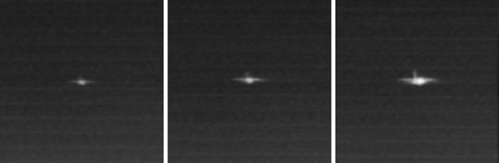
The estimated distances to the target are shown in Figure 2, where $R_A$ is distance obtained on the basis of changes in the target size, the $R_I$ is calculated based on changes in the targets intensity, the $R_C$ is estimated from changes in target contrast from the background, and $R$ is reference range from the DOPRS. All methods perform well and are stable.

The average relative error is calculated by:
IR sequence B
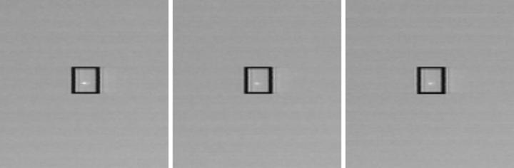
Figure 4 shows the estimated distances to the target using the three algorithms. From the figure one can see that the estimated distance $R_A$ is significantly different than the reference distance $R$. The average relative error is $\overline{Err_{A}}=$12.41%, while it’s maximum value even $Err_{A\max}=$30.78%. Distance estimation error of the other two algorithms is about the same as in the previous scenario, $\overline{Err_{I}}=$1.60%, $\overline{Err_{C}}=$1.86%.

Large error in $R_A$ estimation is a consequence of poor target size estimation. Figure 5 shows the target size, which vary from 3 to 10 pixels.

IR sequence C
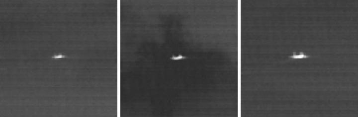
The estimated distances in this sequence are shown in Figure 7, and average error of distances estimations are illustrated in Figure 8. Figure 8 shows a good comparison between range estimations and the reference data at the beginning and the end of sequence, with significant deviations from 100 to 170 frames. This can be explained by an influence of large background changes to the object contrast.


IR sequence D
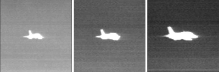
In Figure 10 the estimated distances are shown. The figure shows that the distance $R_A$ sufficiently assess in relation to the reference distance $R$ with the average distance estimation error at $\overline{Err_{A}}=$3.64%. Significant deviation of distance $R_I$ compared to $R$ can be explained by the high intensity of target gray level, due to it proximity.

The average gray level of the target’s pixels is relatively high (94%) and it is more or less constant, which can be explained by saturation of the sensor. The effect of sensor saturation were compensated by the changes of the background gray levels, and the distance estimation $R_C$ is significantly better than the $R_I$.
4 Conclusion
Three monocular passive ranging methods were discussed and applied on four real sequences recorded by an IR sensor. It is shown that these methods offer useful, but not ideal range estimations. Method based on image size measurement requires an extended target (represented with multiple pixels) for acceptable results, although in case of point target (large distances) it generates poor estimations. On the other hand, methods relied on Beer-Lambert's Law give satisfactory results for point target range estimation. When target is close to the sensor, saturation effect arises and deviates contrast and intensity based estimations. Background fluctuation additionally affects the ranging. Results obtained and analyzed suggest the use of a hybrid approach with image size, intensity and contrast features all taken into account.References
- Y. Barniv: Error analysis of combined optical-flow and stereo passive ranging, IEEE Transactions on Aerospace and Electronic Systems, 1992, 28(4), pp. 978-989
- R.J. Pieper, A.W. Cooper, and G. Pelegris: Passive range estimation using dual-baseline triangulation. Optical Engineering, 1996, 35, pp. 685
- M. Ito, S. Tsujimichi, and Y. Kosuge: Tracking a three-dimensional moving target with distributed passive sensors using extended Kalman filter. Electronics and Communications in Japan (Part I: Communications), 2001, 84(7), pp. 74-85
- J.Z. Xu, Z.L. Wang, Y.H. Zhao, and X.J. Guo: A distance estimation algorithm based on infrared imaging guided. International Conference on Machine Learning and Cybernetics, 2009, Vol. 4, pp. 2343-2346
- R. Rao, and S. Lee S. 'A video processing approach for distance estimation', Proc. IEEE Int. Conf. on Acoustics, Speech and Signal Processing, Toulouse, France, July 2006, Vol. III, pp. 1192-1195
- D.R. Van Rheeden: Passive range estimation using image size measurements. US Patent 5,867,256. February, 1999.
- C. Raju, S. Zabuawala, S. Krishna, and J. Yadegar: 'A hybrid system for information fusion with application to passive ranging', Proc. of Int. Conf. on Image Processing, Computer Vision and Pattern Recognition, Las Vegas, June 2007, pp. 402-406
- M. De Visser, P.B.W. Schwering, J.F. de Groot, and E.A. Hendriks: Passive range estimation using dual-baseline triangulation. Optical Engineering, 2006, 45, pp. 026402
- J.R. Anderson, M.R. Hawks, K.C. Gross, and G.P. Perram: 'Flight test of an imaging O (Xb) monocular passive ranging instrument', Proceedings of SPIE, Vol. 802005-12, 2011.
- R.A. Vincent, M.R. Hawks: 'Passive ranging of dynamic rocket plumes using infrared and visible oxygen attenuation', Proceedings of SPIE, Vol. 80520D-16, 2011.
- P. Gil, S. Lafuente, S. Maldonado, and FJ Acevedo: Distance estimation from image defocus for video surveillance systems, Electronics Letters, 2004, 40(17), pp. 1047-1049
- G. Witus and S. Hunt: 'Monocular visual ranging', Proceedings of SPIE, Vol. 696204-1, 2008.
- Yang De-gui and Li Xiang: Passive ranging based on IR radiation characteristics. In Vasyl Morozhenko (editor) Infrared Radiation, InTech 2012, pp. 199-214.
- G.D. Dikic, and Z.M. Djurovic: 'Unbiased estimation of atmosphere attenuation coefficient', Electrical Engineering, 2007, 89, pp. 343-347
- W.-H Tsai: 'Moment-preserving thresolding: A new approach',Computer Vision, Graphics, and Image Processing, 1985, 29(3), pp. 377-393