Next: RESULTS AND DISCUSSION
Up: Development prospects and stability
Previous: INTRODUCTION
MODEL AND BASIC PARAMETERS
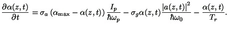
Simulation of the KLM can be based on the two quite different approaches. First one supposes the full-dimensional modelling taking into account the details of the field propagation in the laser cavity [13]. The minimal dimension of such models is 2+1 and the optimization procedure needs mainframe computing. Although this approach allows the description of the spatio-temporal dynamics of the ultrashort pulses and their mode pattern, its main disadvantages are the large number of the parameters resulting in ambiguity of the optimization procedure and complexity of the interpretation of the obtained results. Second approach is based on 1+1 dimensional model in the framework of the so-called nonlinear Ginzburg-Landau equation [14], which describes the KLM as an action of the fast saturable absorber governed by few physically meaningful parameters, viz., its modulation depth
 and the inverse saturation intensity
 . This method allows the analytical realization in the week-nonlinear limit [15], however in the general case the numerical simulations are necessary. We shall be based on the latter approach in view of its physical unambiguity. The master equation describing the ultrashort pulse generation in the KLM solid-state laser is:
 |
(1) |
where
 is the field amplitude (so that
 has a dimension of the intensity),
 is the longitudinal coordinate normalized to the cavity length (thus, as a matter of fact, this is the cavity round-trip number),
 is the local time,
 is the saturated gain coefficient,
 is the linear net-loss coefficient taking into account the intracavity and output losses,
 is the group delay caused by the spectral filtering within the cavity,
 is the
 -order group-delay dispersion (GDD) coefficients,
 =
=
 =
=
 is the self-phase modulation (SPM) coefficient,
 and
and
 are the frequency and wavelength corresponding to the minimum spectral loss,
 and
and
 are the linear and nonlinear refraction coefficients, respectively,
 is the double length of the gain medium (we suppose that the gain medium gives a main contribution to the SPM). The last term in Eq. (
![[*]](crossref.gif) ) describes the self-steepening effect and for the simplification will be not taken into account in the simulations. As an additional simplification we neglect the stimulated Raman scattering in the active medium [16]. These two factors will be considered hereafter. The gain coefficient obeys the following equation:
) describes the self-steepening effect and for the simplification will be not taken into account in the simulations. As an additional simplification we neglect the stimulated Raman scattering in the active medium [16]. These two factors will be considered hereafter. The gain coefficient obeys the following equation:
 |
(2) |
Here
 and
and
 are the absorption and emission cross-sections of the active medium, respectively,
 is the gain relaxation time,
 is the absorbed pump intensity,
  is the pump frequency,
 =
=
 is the maximum gain coefficient,
 is the concentration of the active centers. The assumption
 (
( is the pulse duration,
 is the cavity period) allows the integration of Eq. (
![[*]](http://www.geocities.com/optomaplev/texts/znse/crossref.png) ). Then for the steady-state gain coefficient we have:
). Then for the steady-state gain coefficient we have:
 |
(3) |
where
 =
=
 is the gain saturation energy flux,
 =
=
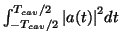 is the pulse energy. For the numerical simulations it is convenient to normalize the time and the intensity to
=
is the pulse energy. For the numerical simulations it is convenient to normalize the time and the intensity to
=
 and
and
 , respectively (
 is the gain bandwidth). The simulation were performed on the
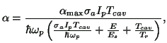
 mesh. Only steady-state pulses were considered. As the criterion of the steady-state operation we chose the peak intensity change less than 1% over last 1000 cavity transits. The KLM in the considered model is governed by only four basic parameters:
 ,
,
 ,
, and
. This allows unambiguous multiparametric optimization. In the presence of the higher-order GDD, the additional
parameters appear. This complicates the optimization procedure, but keeps its physical clarity. Now let us to give the basic material parameters governing the femtosecond oscillation in the lasers under consideration.
,
, and
. This allows unambiguous multiparametric optimization. In the presence of the higher-order GDD, the additional
parameters appear. This complicates the optimization procedure, but keeps its physical clarity. Now let us to give the basic material parameters governing the femtosecond oscillation in the lasers under consideration.
Table:
Material parameters of the Cr-doped Zinc-chalcogenides.
| Medium |
,
 m m |
, nm |
 ,
m ,
m |
, 10 cm cm |
, 10 cm |
|
, 10 esu esu |
,
s |
| Cr:ZnSe |
2.5 |
880 |
1.61 |
8.7 |
9 |
2.44 |
170 |
6-8 |
| Cr:ZnS |
2.35 |
800 |
1.61 |
5.2 |
7.5 |
2.3 |
48 |
4-11 |
| Cr:ZnTe |
2.6 |
800 |
1.61 |
12 |
20 |
2.71 |
830 |
3 |
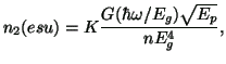
It should be noted that the
values correspond to
, but the experimentally observed
correspond to
 =1.06 m (see Ref. [17]). As a result, we need the theoretical estimation of their values at the generation wavelength. Such estimation can be obtained from the formula [17]:
where
=1.06 m (see Ref. [17]). As a result, we need the theoretical estimation of their values at the generation wavelength. Such estimation can be obtained from the formula [17]:
where
 = (0.5 - 1.5)
 and
and
 = 21 eV are the material independent constants,
 is the band-gap width in eV,
 is the form-factor. Using for
the value, which produces the best agreement with the experimental values of , we can obtain the following estimations:
is the form-factor. Using for
the value, which produces the best agreement with the experimental values of , we can obtain the following estimations:
Table:
Estimations of
at
.
| |
ZnSe |
ZnS |
ZnTe |
|
, 10 esu |
82 |
25 |
380 |
We note that the semiconductor nature of the considered active media results in the extremely high nonlinear refraction coefficients in the comparison with Ti:sapphire, for example (1.2
 esu). As it will be shown below, this has a pronounced manifestation in the femtosecond pulse dynamics. The simulation parameters corresponding to the above introduced normalizations are summarized in Table (
 ,
,
 =
=
 ).
).
Table:
Simulation parameters.
=2 0.3 cm, =10 ns, 2 W pump power, 100100
m pump mode.
0.3 cm, =10 ns, 2 W pump power, 100100
m pump mode.
| Medium |
|
, 10 cm/W cm/W |
, 10 cm/W cm/W |
, 10 |
, fs |
P, 10 |
| Cr:ZnSe |
5 |
141 |
87 |
4.9 |
3.8 |
1.1 |
| Cr:ZnS |
5 |
45.5 |
32 |
10 |
3.7 |
0.62 |
| Cr:ZnTe |
5 |
587 |
314 |
3.8 |
4.5 |
1.9 |
Next: RESULTS AND DISCUSSION
Up: Development prospects and stability
Previous: INTRODUCTION
V.L. Kalashnikov
2002-12-28