![E = (e[t]+e[z])*exp(i*beta*z)](images/TFmodes1.gif) ,
,
![H = (h[t]+h[z])*exp(i*beta*z)](images/TFmodes2.gif) , where
, where
Effective refractive indexes and dispersion characteristics of the tapered fibers
Vladimir L. Kalashnikov
Institut fuer Photonik, TU Wien, Gusshausstrasse 27/387, A-1040 Vienna, Austria
http://www.geocities.com/optomaplev
Abstract: Analytical consideration of the circular and rectangular step-profile fibers is presented. The Helmholtz's equation for a fiber mode results in the transcendental equation for the propagation constant, which can be solved numerically by means of the Matlab-procedure. As a result, the effective refractivity indexes and the fiber's dispersion can be obtained.
Application Areas/Subjects : Fiber Optics, Differential Equations, and Programming.
Keywords: tapered fiber, fiber mode, Helmholtz's equation.
The tapered fibers, i.e. the fibers are fabricated by heating and stretching standard fiber in a flame or by extruding porous fiber and providing a high degree of the light localization, are of great interest for the novel light sources (for review see, P. Russell , "Photonic crystal fibers", Nature , 299 , 358-362 (2003).). A strong and controlled contribution of the air to the fiber dispersion as well as the high intra-fiber light intensity cause the spectral continua generation.
Here we shall analyze the tapered fiber dispersion on the basis of the simple analytical models described in A.Snyder, J.Love "Optical Waveguide theory" (Chapman and Hall, 1983) and D.Marcuse "Theory of dielectric optical waveguides" (Academic Press, 1974) .
The basic equation describing the monochromatic mode of the translationally invariant fiber is the Helmholtz's equation. Let's decompose the electric and magnetic fields in the following form:
,
, where
![]() (
(
![]() ) are the transverse (to the propagation axis
z
) vector field components,
) are the transverse (to the propagation axis
z
) vector field components,
![]() (
(
![]() ) are the longitudinal field components,
) are the longitudinal field components,
![]() is the propagation constant defining the effective refractive index for the propagating mode (we eliminated the time-dependence for the monochromatic mode). For the homogeneous fiber (core) embedded in the air surroundings (cladding) we can solve the Helmholtz's equation for core and cladding separately and then to impose the continuity of the field components on the interface.
is the propagation constant defining the effective refractive index for the propagating mode (we eliminated the time-dependence for the monochromatic mode). For the homogeneous fiber (core) embedded in the air surroundings (cladding) we can solve the Helmholtz's equation for core and cladding separately and then to impose the continuity of the field components on the interface.
Circular waveguide
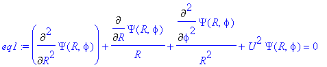
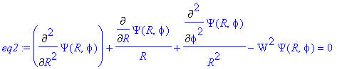
| > | restart: with('linalg'): with(stats): with(plots): # CIRCULAR WAVEGUIDE # k is the vacuum wave number; # rho is the fiber radius; # R=r/rho; # r is the radial coordinate; # phi is the azimuth coordinate; # n[co] is the core's refractive index; # n[cl] is the cladding's refractive index; # Psi = (e[z],h[z]). c1 := U = rho*sqrt(k^2*n[co]^2-beta^2); c2 := W = rho*sqrt(beta^2-k^2*n[cl]^2); print(`FIBER:`); eq1 := Diff(Psi(R,phi),R$2) + Diff(Psi(R,phi),R)/R + Diff(Psi(R,phi),phi$2)/R^2 + U^2*Psi(R,phi) = 0; print(`AIR:`); eq2 := Diff(Psi(R,phi),R$2) + Diff(Psi(R,phi),R)/R + Diff(Psi(R,phi),phi$2)/R^2 - W^2*Psi(R,phi) = 0; |
Warning, the protected names norm and trace have been redefined and unprotected
Warning, the name changecoords has been redefined
![]()
![]()
![]()
![]()
We can separate the radial and azimuthal variables:
| > | Psi(R,phi)=psi(R)*cos(nu*phi); subs( %,eq1 ): eq3 := expand( value(%)/cos(nu*phi) ); print(`alternative form:`); Psi(R,phi)=psi(R)*sin(nu*phi); subs( %,eq1 ): eq4 := expand( value(%)/sin(nu*phi) ); |
![]()

![]()
![]()

The obvious solution is:
| > | sol1 := dsolve(eq3); |
![]()
Since
| > | limit(BesselY(0,x),x=0); |
![]()
a regularity of solution requires:
| > | sol[1] := subs({_C2=0,_C1=C/BesselJ(nu,U)},sol1); #regularity at center. C is some constant |
![]()
In like manner for the air:
| > | Psi(R,phi)=psi(R)*cos(nu*phi); subs( %,eq2 ): eq5 := expand( value(%)/cos(nu*phi) ); print(`alternative form:`); Psi(R,phi)=psi(R)*sin(nu*phi); subs( %,eq2 ): eq6 := expand( value(%)/sin(nu*phi) ); |
![]()
![]()
![]()
The solution is:
| > | sol3 := dsolve(eq5); |
![]()
Regularity at infinity requires:
| > | # Since limit(BesselI(0,x),x=infinity); sol[2] := subs({_C1=0,_C2=C/BesselK(nu,W)},sol3); #regularity at infinity |
![]()
![]()
Hence, we have for the longitudinal field components:
| > | print(`Electric field in core:`); ez[1,even] := subs( C=A,rhs(sol[1])*cos(nu*phi) );# core, even mode ez[1,odd] := subs( C=A,rhs(sol[1])*sin(nu*phi) );# core, odd mode print(`Magnetic field in core:`); hz[1,even] := subs( C=B,rhs(sol[1])*(-sin(nu*phi)) );# core, even mode hz[1,odd] := subs( C=B,rhs(sol[1])*cos(nu*phi) );# core, odd mode print(`Electric field in cladding:`); ez[2,even] := subs( C=A,rhs(sol[2])*cos(nu*phi) );# cladding, even mode ez[2,odd] := subs( C=A,rhs(sol[2])*sin(nu*phi) );# cladding, odd mode print(`Magnetic field in cladding:`); hz[2,even] := subs( C=B,rhs(sol[2])*(-sin(nu*phi)) );# cladding, even mode hz[2,odd] := subs( C=B,rhs(sol[2])*cos(nu*phi) );# cladding, odd mode |
![]()
![]()
![]()
![]()
![]()
![]()
![]()
![]()
![]()
![]()
![]()
![]()
The transverse field components can be expressed through the longitudinal ones (the Maple-based deviation from the Maxwell's equations will be presented elsewhere):
| > | f1 := e[phi] = I/p*( beta/R*diff(e[z](R,phi),phi)-sqrt(mu0/epsilon0)*k*diff(h[z](R,phi),R) ); f2 := h[phi] = I/p*( beta/R*diff(h[z](R,phi),phi)+sqrt(epsilon0/mu0)*k*n^2*diff(e[z](R,phi),R) ); |
![f1 := e[phi] = 1/p*(beta/R*diff(e[z](R,phi),phi)-(mu0/epsilon0)^(1/2)*k*diff(h[z](R,phi),R))*I](images/TFmodes42.gif)
![f2 := h[phi] = 1/p*(beta/R*diff(h[z](R,phi),phi)+(epsilon0/mu0)^(1/2)*k*n^2*diff(e[z](R,phi),R))*I](images/TFmodes43.gif)
| > | print(`Core:`); eq7 := value( subs({e[z](R,phi)=ez[1,even],h[z](R,phi)=hz[1,even]},rhs(f1)) );# electric field in core; even mode eq8 := value( subs({e[z](R,phi)=ez[1,even],h[z](R,phi)=hz[1,even]},rhs(f2)) );# magnetic field in core; even mode eq9 := value( subs({e[z](R,phi)=ez[1,odd],h[z](R,phi)=hz[1,odd]},rhs(f1)) );# electric field in core; odd mode eq10 := value( subs({e[z](R,phi)=ez[1,odd],h[z](R,phi)=hz[1,odd]},rhs(f2)) );# magnetic field in core; odd mode print(`Cladding:`); eq11 := value( subs({e[z](R,phi)=ez[2,even],h[z](R,phi)=hz[2,even]},rhs(f1)) );# electric field in cladding; even mode eq12 := value( subs({e[z](R,phi)=ez[2,even],h[z](R,phi)=hz[2,even]},rhs(f2)) );# magnetic field in cladding; even mode eq13 := value( subs({e[z](R,phi)=ez[2,odd],h[z](R,phi)=hz[2,odd]},rhs(f1)) );# electric field in cladding; odd mode eq14 := value( subs({e[z](R,phi)=ez[2,odd],h[z](R,phi)=hz[2,odd]},rhs(f2)) );# magnetic field in cladding; odd mode |
![]()
![]()

Where
| > | eq15 := p = k^2*n^2-beta^2; |
![]()
Continuity on interface ( R =1) requires:
| > | eq16 := expand( subs( n=n[co],subs( {eq15,R=1},eq7 ) )/I/sin(nu*phi) = subs( n=n[cl],subs( {eq15,R=1},eq11 ) )/I/sin(nu*phi)); eq17 := expand( subs( n=n[co],subs( {eq15,R=1},eq8 ) )/I/cos(nu*phi) = subs( n=n[cl],subs( {eq15,R=1},eq12 ) )/I/cos(nu*phi) ); |
![]()
![eq16 := -1/(k^2*n[co]^2-beta^2)*beta*A*nu-1/(k^2*n[co]^2-beta^2)*(mu0/epsilon0)^(1/2)*k*B/BesselJ(nu,U)*U*BesselJ(nu+1,U)+1/(k^2*n[co]^2-beta^2)*(mu0/epsilon0)^(1/2)*k*B*nu = -1/(k^2*n[cl]^2-beta^2)*be...](images/TFmodes56.gif)
![eq17 := -1/(k^2*n[co]^2-beta^2)*beta*B*nu-1/(k^2*n[co]^2-beta^2)*(epsilon0/mu0)^(1/2)*k*n[co]^2*A/BesselJ(nu,U)*U*BesselJ(nu+1,U)+1/(k^2*n[co]^2-beta^2)*(epsilon0/mu0)^(1/2)*k*n[co]^2*A*nu = -1/(k^2*n[...](images/TFmodes57.gif)
![eq17 := -1/(k^2*n[co]^2-beta^2)*beta*B*nu-1/(k^2*n[co]^2-beta^2)*(epsilon0/mu0)^(1/2)*k*n[co]^2*A/BesselJ(nu,U)*U*BesselJ(nu+1,U)+1/(k^2*n[co]^2-beta^2)*(epsilon0/mu0)^(1/2)*k*n[co]^2*A*nu = -1/(k^2*n[...](images/TFmodes58.gif)
Hence:
| > | eq19 := subs({k^2*n[co]^2-beta^2=U^2/rho^2,k^2*n[cl]^2-beta^2=-W^2/rho^2},eq16); eq20 := subs({k^2*n[co]^2-beta^2=U^2/rho^2,k^2*n[cl]^2-beta^2=-W^2/rho^2},eq17); |

![eq20 := -1/U^2*rho^2*beta*B*nu-1/U*rho^2*(epsilon0/mu0)^(1/2)*k*n[co]^2*A/BesselJ(nu,U)*BesselJ(nu+1,U)+1/U^2*rho^2*(epsilon0/mu0)^(1/2)*k*n[co]^2*A*nu = 1/W^2*rho^2*beta*B*nu+1/W*rho^2*(epsilon0/mu0)^...](images/TFmodes60.gif)
![eq20 := -1/U^2*rho^2*beta*B*nu-1/U*rho^2*(epsilon0/mu0)^(1/2)*k*n[co]^2*A/BesselJ(nu,U)*BesselJ(nu+1,U)+1/U^2*rho^2*(epsilon0/mu0)^(1/2)*k*n[co]^2*A*nu = 1/W^2*rho^2*beta*B*nu+1/W*rho^2*(epsilon0/mu0)^...](images/TFmodes61.gif)
Let us perform some manipulations to exclude constants A and B .
| > | eq21 := expand((lhs(eq19) - rhs(eq19))/rho^2); eq22 := expand((lhs(eq20) - rhs(eq20))/rho^2); |
![eq22 := -1/U^2*beta*B*nu-1/U*(epsilon0/mu0)^(1/2)*k*n[co]^2*A/BesselJ(nu,U)*BesselJ(nu+1,U)+1/U^2*(epsilon0/mu0)^(1/2)*k*n[co]^2*A*nu-1/W^2*beta*B*nu-1/W*(epsilon0/mu0)^(1/2)*k*n[cl]^2*A/BesselK(nu,W)*...](images/TFmodes63.gif)
| > | eq23 := expand( eq21/B ); eq24 := expand( eq22/A ); |
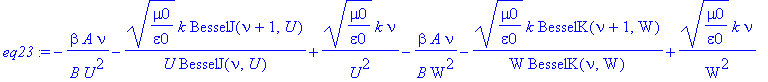
![eq24 := -1/A/U^2*beta*B*nu-1/U*(epsilon0/mu0)^(1/2)*k*n[co]^2/BesselJ(nu,U)*BesselJ(nu+1,U)+1/U^2*(epsilon0/mu0)^(1/2)*k*n[co]^2*nu-1/A/W^2*beta*B*nu-1/W*(epsilon0/mu0)^(1/2)*k*n[cl]^2/BesselK(nu,W)*Be...](images/TFmodes65.gif)
| > | collect(eq23,A): eq25 := A/B = -(% - coeff(%,A)*A)/expand( coeff(%,A)*B ); |
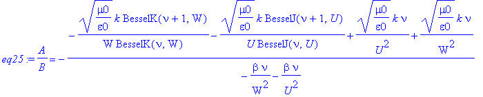
| > | collect(eq24,B): eq26 := B/A = -(% - coeff(%,B)*B)/expand( coeff(%,B)*A ); |
![eq26 := B/A = -(-1/W*(epsilon0/mu0)^(1/2)*k*n[cl]^2/BesselK(nu,W)*BesselK(nu+1,W)-1/U*(epsilon0/mu0)^(1/2)*k*n[co]^2/BesselJ(nu,U)*BesselJ(nu+1,U)+1/U^2*(epsilon0/mu0)^(1/2)*k*n[co]^2*nu+1/W^2*(epsilon...](images/TFmodes67.gif)
Thus, from eq25 and eq26 we have:
| > | 1/rhs(eq26) = rhs(eq25): rhs(eq25)*rhs(eq26) = 1: eq27 := lhs(%)*(-1/W^2*beta*nu-1/U^2*beta*nu)^2/k^2/n[co]^2 = simplify( (-1/W^2*beta*nu-1/U^2*beta*nu)^2/k^2/n[co]^2 ); |
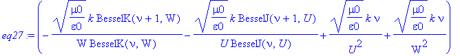

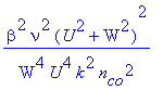
The left hand-side can be expressed as follows:
| > | eq28 := ((-BesselJ(nu+1,U)+nu/U*BesselJ(nu,U))/U/BesselJ(nu,U)+(-BesselK(nu+1,W)+nu/W*BesselK(nu,W))/W/BesselK(nu,W))*((-BesselJ(nu+1,U)+nu/U*BesselJ(nu,U))/U/BesselJ(nu,U)+n[cl]^2/n[co]^2*(-BesselK(nu+1,W)+nu/W*BesselK(nu,W))/W/BesselK(nu,W)); print(`equality check:`); simplify(simplify( lhs(eq27),power, symbolic) - simplify(eq28) ); |
![eq28 := ((-BesselJ(nu+1,U)+nu/U*BesselJ(nu,U))/U/BesselJ(nu,U)+(-BesselK(nu+1,W)+nu/W*BesselK(nu,W))/W/BesselK(nu,W))*((-BesselJ(nu+1,U)+nu/U*BesselJ(nu,U))/U/BesselJ(nu,U)+n[cl]^2/n[co]^2*(-BesselK(nu...](images/TFmodes71.gif)
![eq28 := ((-BesselJ(nu+1,U)+nu/U*BesselJ(nu,U))/U/BesselJ(nu,U)+(-BesselK(nu+1,W)+nu/W*BesselK(nu,W))/W/BesselK(nu,W))*((-BesselJ(nu+1,U)+nu/U*BesselJ(nu,U))/U/BesselJ(nu,U)+n[cl]^2/n[co]^2*(-BesselK(nu...](images/TFmodes72.gif)
![]()
![]()
Finally, we have the equation for the propagation constant:
| > | res := eq28 = rhs(eq27); |
![res := ((-BesselJ(nu+1,U)+nu/U*BesselJ(nu,U))/U/BesselJ(nu,U)+(-BesselK(nu+1,W)+nu/W*BesselK(nu,W))/W/BesselK(nu,W))*((-BesselJ(nu+1,U)+nu/U*BesselJ(nu,U))/U/BesselJ(nu,U)+n[cl]^2/n[co]^2*(-BesselK(nu+...](images/TFmodes75.gif)
![res := ((-BesselJ(nu+1,U)+nu/U*BesselJ(nu,U))/U/BesselJ(nu,U)+(-BesselK(nu+1,W)+nu/W*BesselK(nu,W))/W/BesselK(nu,W))*((-BesselJ(nu+1,U)+nu/U*BesselJ(nu,U))/U/BesselJ(nu,U)+n[cl]^2/n[co]^2*(-BesselK(nu+...](images/TFmodes76.gif)
The last equation can be solved by Matlab-procedures (files
f1.m and
tap_f1.m). The basic function is
tap_f1
(x
)
whose argument is the tapered fiber radius in meters. The result is the effective refractive index for the fundamental mode in the spectral range of 0.22 - 3.21
![]() m (we supposed that the fiber's material is the fused silica). The obtained result is written in the file
neff1.dat
(the fiber diameter is 1.5
m (we supposed that the fiber's material is the fused silica). The obtained result is written in the file
neff1.dat
(the fiber diameter is 1.5
![]() m). The effective refractive index and its fitting are shown below in the comparison with the refractivity of the bulk material.
m). The effective refractive index and its fitting are shown below in the comparison with the refractivity of the bulk material.
| > | neff := readdata(`neff1.dat`,2,float): n_bulk := readdata(`bulk1.dat`,2,float): # refractive index of the bulk fused silica for i from 1 to 300 do Q[i] := [neff[i,1],neff[i,2]]: od: for i from 1 to 35 do R[i] := [n_bulk[i,1],n_bulk[i,2]]: od: p1 := statplots[scatterplot]([Q[k][1] $k=1..300],[Q[k][2] $k=1..300]): eq29 := fit[leastsquare[[x,y], y=a0+a1*x^2+a2/x^2+a3/x^4+a4/x^6+a5/x^8+b/x+c*x+d*x^3+e/x^3+f*x^9+g/x^9+h*x^10+hh/x^10,{a0,a1,a2,a3,a4,a5,b,c,d,e,f,g,h,hh}]]([[Q[k][1] $k=1..300],[Q[k][2] $k=1..300]]): p2 := plot(rhs(eq29),x=0.21..3.4,color=green): p3 := statplots[scatterplot]([R[k][1] $k=1..35],[R[k][2] $k=1..35]): eq30 := fit[leastsquare[[x,y], y=a0+a1*x^2+a2/x^2+a3/x^4+a4/x^6+a5/x^8+b/x+c*x+d*x^3+e/x^3+f*x^9+g/x^9+h*x^10+hh/x^10,{a0,a1,a2,a3,a4,a5,b,c,d,e,f,g,h,hh}]]([[R[k][1] $k=1..35],[R[k][2] $k=1..35]]): p4 := plot(rhs(eq30),x=0.21..3.4,color=red): display(p1,p2,p3,p4,axes=boxed,title=`refractive index vs. wavelength (in mkm)`); |
![[Maple Plot]](images/TFmodes79.gif)
The group-delay and group-velocity dispersions can be obtained from eq29 :
| > | eq31 := subs(c=299792458e-15,x^3*diff( rhs(eq29), x$2)*1e-9/c^2/(2*Pi)): eq32 := subs(c=299792458e-15,x^3*diff( rhs(eq30), x$2)*1e-9/c^2/(2*Pi)): d1 := plot( eq31,x=0.4..3.4,color=blue): d2 := plot( eq32,x=0.4..3.4,color=red): display(d1,d2,axes=boxed,view=-500..500,title=`GDD, ps^2/km`); eq33 := -2*Pi*eq31*299792458*1e-3/(1e6*x^2): eq34 := -2*Pi*eq32*299792458*1e-3/(1e6*x^2): d3 := plot( eq33,x=0.4..3,color=blue): d4 := plot( eq34,x=0.4..3,color=red): display(d3,d4,view=-400..300,axes=boxed,title=`GVD, ps/km/nm`); |
![[Maple Plot]](images/TFmodes80.gif)
![[Maple Plot]](images/TFmodes81.gif)
Rectangular waveguide
For the rectangular waveguide imbedded in the air cladding, we have:
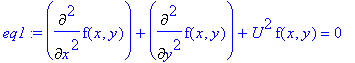
| > | restart: with('linalg'): with(stats): with(plots): with(PDEtools): # RECTANGULAR WAVEGUIDE (core is a (b x d)-rectangle, its left-upper corner corresponds to x=y=0) print(`HELMHOLTZ's EQUATION for e[z] and h[z] components:`); eq1 := Diff(f(x,y),x$2) + Diff(f(x,y),y$2) + U^2*f(x,y) = 0;# U^2=n^2*k^2-beta^2 = k_x^2+k_y^2 print(`from the Maxwell's equations:`); f3 := e[x] = -I/U^2*( beta*diff(e[z](x,y),x)+(mu0*omega)*diff(h[z](x,y),y) ); f4 := e[y] = -I/U^2*( beta*diff(e[z](x,y),y)-(mu0*omega)*diff(h[z](x,y),x) ); f5 := h[x] = -I/U^2*( beta*diff(h[z](x,y),x)-(n^2*epsilon0*omega)*diff(e[z](x,y),y) ); f6 := h[y] = -I/U^2*( beta*diff(h[z](x,y),y)+(n^2*epsilon0*omega)*diff(e[z](x,y),x) ); |
Warning, the protected names norm and trace have been redefined and unprotected
Warning, the name changecoords has been redefined
![]()
![]()
![f3 := e[x] = -I/U^2*(beta*diff(e[z](x,y),x)+mu0*omega*diff(h[z](x,y),y))](images/TFmodes85.gif)
![f4 := e[y] = -I/U^2*(beta*diff(e[z](x,y),y)-mu0*omega*diff(h[z](x,y),x))](images/TFmodes86.gif)
![f5 := h[x] = -I/U^2*(beta*diff(h[z](x,y),x)-n^2*epsilon0*omega*diff(e[z](x,y),y))](images/TFmodes87.gif)
![f6 := h[y] = -I/U^2*(beta*diff(h[z](x,y),y)+n^2*epsilon0*omega*diff(e[z](x,y),x))](images/TFmodes88.gif)
![]() -modes
-modes
The symmetry of the core suggests an existence of the two types of modes: i) polarized in x-direction (vertical axis, x-modes) and ii) polarized in y-direction (horizontal axis, y-modes).
In the beginning, let's consider x-modes .
eq1 allows the separation of variables:
| > | sol := pdsolve(eq1); |
![sol := `&where`(f(x,y) = _F1(x)*_F2(y),[{diff(_F1(x),`$`(x,2)) = _c[1]*_F1(x), diff(_F2(y),`$`(y,2)) = -_c[1]*_F2(y)-U^2*_F2(y)}])](images/TFmodes90.gif)
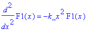
| > | diff(F1(x),`$`(x,2)) = -k_x^2*F1(x); # _c[1]=-k_x^2, k_x is the x-projection of the wave vector sol1 := dsolve(%); diff(F2(y),`$`(y,2)) = -k_y^2*F2(y);# k_y is the y-projection of the wave vector sol2 := dsolve(%); |
![]()

![]()
Hence, the general solution is:
| > | sol := simplify( rhs(sol1)*rhs(sol2) ); |
![]()
Then, the electric field can be expressed as (we introduced the phase parameters
![]() and
and
![]() instead of the constants of integration):
instead of the constants of integration):
| > | eq2 := e[z](x,y) = A*cos(k_x*(x+xi))*cos(k_y*(y+eta)); |
![]()
By definition
, x-mode
requires
![]() . Hence,
. Hence,
| > | expand( -numer(rhs(f5))/I/beta ) = 0; value( subs(eq2,%) ); dsolve(%,h[z](x,y)); |
,x)-1/beta*n^2*epsilon0*omega*diff(e[z](x,y),y) = 0](images/TFmodes100.gif)
,x)+1/beta*n^2*epsilon0*omega*A*cos(k_x*(x+xi))*sin(k_y*(y+eta))*k_y = 0](images/TFmodes101.gif)
 = -n^2*sin(k_y*(y+eta))*k_y*epsilon0/beta*omega*A/k_x*sin(k_x*x+k_x*xi)+_F1(y)](images/TFmodes102.gif)
For reasons of symmetry,
![]() . Then
. Then
| > | eq3 := h[z](x,y) = -A*n^2*(k_y/k_x)*(k/beta)*sqrt(epsilon0/mu0)*sin(k_x*(x+xi))*sin(k_y*(y+eta)); # k = omega*sqrt(epsilon0*mu0) is the vacuum wave number |
 = -A*n^2*k_y/k_x*k/beta*(epsilon0/mu0)^(1/2)*sin(k_x*(x+xi))*sin(k_y*(y+eta))](images/TFmodes104.gif)
eq2 and eq3 result in:
| > | subs({eq2,eq3},f3): eq4 := simplify(%); subs({eq2,eq3},f4): eq5 := simplify(%); subs({eq2,eq3},f6): eq6 := simplify(%); |
![eq4 := e[x] = A*sin(k_x*(x+xi))*cos(k_y*(y+eta))*(beta^2*k_x^2+mu0*omega*n^2*k_y^2*k*(epsilon0/mu0)^(1/2))/U^2/beta/k_x*I](images/TFmodes105.gif)
![eq5 := e[y] = -I*A*cos(k_x*(x+xi))*sin(k_y*(y+eta))*k_y*(-beta^2+mu0*omega*n^2*k*(epsilon0/mu0)^(1/2))/U^2/beta](images/TFmodes106.gif)
![eq6 := h[y] = A*n^2*sin(k_x*(x+xi))*cos(k_y*(y+eta))*(k_y^2*k*(epsilon0/mu0)^(1/2)+epsilon0*omega*k_x^2)/U^2/k_x*I](images/TFmodes107.gif)
Hence
| > | subs({k=omega*sqrt(epsilon0*mu0),U=sqrt(k_x^2+k_y^2)},eq6): simplify(%,radical,symbolic): eq7 := subs(omega=k/sqrt(epsilon0*mu0),%); subs(U=sqrt(-beta^2+k^2*n^2),eq5): simplify(%,radical,symbolic): eq8 := subs(omega=k/sqrt(epsilon0*mu0),%); simplify(eq4,radical,symbolic): eq9 := subs(omega=k/sqrt(epsilon0*mu0),%); |
![eq7 := h[y] = epsilon0*k/(epsilon0*mu0)^(1/2)*cos(k_y*(y+eta))*sin(k_x*(x+xi))*n^2*A/k_x*I](images/TFmodes108.gif)
![]()
![eq9 := e[x] = A*sin(k_x*(x+xi))*cos(k_y*(y+eta))*(beta^2*k_x^2+k^2*n^2*k_y^2)/U^2/beta/k_x*I](images/TFmodes110.gif)
The last expression can be transformed by virtue of the following equalities:
| > | k_y^2 = n^2*k^2 - k_x^2 - beta^2; beta^2*k_x^2+k^2*n^2*k_y^2 = rhs(expand( %*k^2*n^2 )) + beta^2*k_x^2; factor(rhs(%)); U^2 = factor(n^2*k^2-beta^2); # Hence eq10 := e[x] = A*sin(k_x*(x+xi))*cos(k_y*(y+eta))*(k^2*n^2-k_x^2)/beta/k_x*I; |
![]()
![]()
![]()
![]()
![eq10 := e[x] = A*sin(k_x*(x+xi))*cos(k_y*(y+eta))*(k^2*n^2-k_x^2)/beta/k_x*I](images/TFmodes115.gif)
| > | print(`Resulting system for core (n=n[co]):`); f7 := eq2; f8 := eq3; f9 := eq10; f10 := h[x](x,y) = 0; f11 := eq8; f12 := eq7; |
![]()
![]()
 = -A*n^2*k_y/k_x*k/beta*(epsilon0/mu0)^(1/2)*sin(k_x*(x+xi))*sin(k_y*(y+eta))](images/TFmodes118.gif)
![f9 := e[x] = A*sin(k_x*(x+xi))*cos(k_y*(y+eta))*(k^2*n^2-k_x^2)/beta/k_x*I](images/TFmodes119.gif)
![]()
![]()
![f12 := h[y] = epsilon0*k/(epsilon0*mu0)^(1/2)*cos(k_y*(y+eta))*sin(k_x*(x+xi))*n^2*A/k_x*I](images/TFmodes122.gif)
Below we shall consider only low-order modes, which have small deviations from the fiber axis. For such modes
![]() ,
,
![]() <<
<<
![]() , i.e. we can neglect
, i.e. we can neglect
![]() . Also, we have to suppose the decay of the field far from the core. Also, we shall take into account a continuity of the tangential electric field component on the interfaces.
. Also, we have to suppose the decay of the field far from the core. Also, we shall take into account a continuity of the tangential electric field component on the interfaces.
For the air sector laying below the rectangular core we can obviously transform the obtained solutions in the agreement with the above mentioned requirements:
| > | f13 := lhs(f7) = subs( x=-d,rhs(f7) )*exp(gamma*(x+d)); value( subs( {f(x,y)=rhs(%),U^2=k_y^2-gamma^2},eq1 ) ):# we introduced the attenuation parameter gamma: U^2=k_y^2-gamma^2. Continuity condition is satisfied simplify(%);# that is solution of the Helmholtz's equation f14 := lhs(f8) = -A*n^2*k_y/gamma*k/beta*(epsilon0/mu0)^(1/2)*cos(k_x*(xi-d))*sin(k_y*(y+eta))*exp(gamma*(x+d)); value( subs( {f(x,y)=rhs(%),U^2=k_y^2-gamma^2},eq1 ) ): simplify(%);# that is solution of the Helmholtz's equation value( subs( {f13,f14,omega=k/sqrt(epsilon0*mu0)},numer(rhs(f5)) ) ): simplify(%,radical,symbolic);# we have to satisfy h[x]=0 |
![]()
![]()
 = -A*n^2*k_y/gamma*k/beta*(epsilon0/mu0)^(1/2)*cos(k_x*(-d+xi))*sin(k_y*(y+eta))*exp(gamma*(x+d))](images/TFmodes129.gif)
![]()
![]()
The remaining projections of the field can be obtained from their longitudinal components.
| > | subs({f13,f14},f3): simplify(%,radical,symbolic): subs(omega=k/sqrt(epsilon0*mu0),%); # As previously, we have some equalities: k_y^2 = n^2*k^2 + gamma^2 - beta^2; -beta^2*gamma^2+k^2*n^2*k_y^2 = rhs(expand( %*k^2*n^2 )) - beta^2*gamma^2; factor(rhs(%)); U^2 = factor(n^2*k^2-beta^2); # Hence f15 := e[x](x,y) = I*A*(k^2*n^2+gamma^2)*cos(k_x*(xi-d))*cos(k_y*(y+eta))*exp(gamma*(x+d))/gamma/beta; |
![e[x] = A*cos(k_x*(d-xi))*cos(k_y*(y+eta))*exp(gamma*(x+d))*(-beta^2*gamma^2+k^2*n^2*k_y^2)/U^2/gamma/beta*I](images/TFmodes132.gif)
![]()
![]()
![]()
![]()
 = A*(k^2*n^2+gamma^2)*cos(k_x*(-d+xi))*cos(k_y*(y+eta))*exp(gamma*(x+d))/gamma/beta*I](images/TFmodes137.gif)
| > | subs({f13,f14},f4): simplify(%,radical,symbolic): subs({omega=k/sqrt(epsilon0*mu0),U=sqrt(k^2*n^2-beta^2)},%);# this is zero by virtue of our approximation k_y<<beta subs({f13,f14},f6): simplify(%,radical,symbolic): subs(omega=k/sqrt(epsilon0*mu0),%): simplify(%,radical,symbolic); f16 := h[y](x,y) = -subs(U=sqrt(-k_y^2+gamma^2),rhs(%)); |
![e[y] = -I*A*cos(k_x*(d-xi))*sin(k_y*(y+eta))*k_y*exp(gamma*(x+d))/beta](images/TFmodes138.gif)
![h[y] = -I*A*n^2*cos(k_x*(d-xi))*cos(k_y*(y+eta))*exp(gamma*(x+d))*k*epsilon0*(-k_y^2+gamma^2)/(epsilon0*mu0)^(1/2)/U^2/gamma](images/TFmodes139.gif)
 = A*n^2*cos(k_x*(d-xi))*cos(k_y*(y+eta))*exp(gamma*(x+d))*k*epsilon0/(epsilon0*mu0)^(1/2)/gamma*I](images/TFmodes140.gif)
So, we have the system for the lower air sector:
| > | print(`Resulting system for lower air sector (n=n[cl]):`); f13; f14; f15; f10; f17 := e[y](x,y) = 0; f16; |
![]()
![]()
 = -A*n^2*k_y/gamma*k/beta*(epsilon0/mu0)^(1/2)*cos(k_x*(-d+xi))*sin(k_y*(y+eta))*exp(gamma*(x+d))](images/TFmodes143.gif)
 = A*(k^2*n^2+gamma^2)*cos(k_x*(-d+xi))*cos(k_y*(y+eta))*exp(gamma*(x+d))/gamma/beta*I](images/TFmodes144.gif)
![]()
![]()
 = A*n^2*cos(k_x*(d-xi))*cos(k_y*(y+eta))*exp(gamma*(x+d))*k*epsilon0/(epsilon0*mu0)^(1/2)/gamma*I](images/TFmodes147.gif)
The coordinate shift and the change of the attenuation parameter's sign allow the system for the upper air sector:
| > | print(`Resulting system for upper air sector (n=n[cl]):`); f18 := subs({d=0,gamma=-gamma},f13); f19 := subs({d=0,gamma=-gamma},f14); f20 := subs({d=0,gamma=-gamma},f15); f10; f17; f21 := subs({d=0,gamma=-gamma},f16); |
![]()
![]()
 = A*n^2*k_y/gamma*k/beta*(epsilon0/mu0)^(1/2)*cos(k_x*xi)*sin(k_y*(y+eta))*exp(-gamma*x)](images/TFmodes150.gif)
 = -I*A*(k^2*n^2+gamma^2)*cos(k_x*xi)*cos(k_y*(y+eta))*exp(-gamma*x)/gamma/beta](images/TFmodes151.gif)
![]()
![]()
 = -I*A*n^2*cos(-k_x*xi)*cos(k_y*(y+eta))*exp(-gamma*x)*k*epsilon0/(epsilon0*mu0)^(1/2)/gamma](images/TFmodes154.gif)
Now let's consider the right air sector and demand the continuity of
![]() -component.
-component.
| > | eq11 := e[x](x,y) = subs({y=b,A=B},rhs(f9))*exp(-gamma*(y-b));# air, B is some constant subs(n=n[cl],f9);# core simplify( subs({y=b,n=n[cl]},rhs(eq11)) ) = simplify( subs({y=b,n=n[co]},rhs(f9)) ): eq12 := B = solve(%,B); |
 = B*sin(k_x*(x+xi))*cos(k_y*(b+eta))*(k^2*n^2-k_x^2)/beta/k_x*exp(-gamma*(y-b))*I](images/TFmodes156.gif)
![e[x] = A*sin(k_x*(x+xi))*cos(k_y*(y+eta))*(k^2*n[cl]^2-k_x^2)/beta/k_x*I](images/TFmodes157.gif)
![eq12 := B = A*(k^2*n[co]^2-k_x^2)/(k^2*n[cl]^2-k_x^2)](images/TFmodes158.gif)
For the low-order modes we can neglect
![]() in comparison with
in comparison with
![]() . Hence:
. Hence:
| > | subs(k_x=0,eq12); f22 := subs({%,n=n[cl]},eq11); |
![B = A*n[co]^2/n[cl]^2](images/TFmodes161.gif)
 = A*n[co]^2/n[cl]^2*sin(k_x*(x+xi))*cos(k_y*(b+eta))*(k^2*n[cl]^2-k_x^2)/beta/k_x*exp(-gamma*(y-b))*I](images/TFmodes162.gif)
Now we shall consider z-components of the fields and adjust their amplitudes through
f22
and
![]() .
.
| > | eq13 := C*cos(k_x*(x+xi))*cos(k_y*(b+eta))*exp(-gamma*(y-b));# e[z] eq14 := D*sin(k_x*(x+xi))*cos(k_y*(b+eta))*exp(-gamma*(y-b));# h[z] subs({e[z](x,y)=eq13,h[z](x,y)=eq14},rhs(f5)):# h[x] subs({omega=k/sqrt(epsilon0*mu0),n=n[cl]},numer(%)): simplify(%,radical,symbolic): numer(%); |
![]()
![]()
![]()
So, we have the equations for the adjusting constants:
| > | eq15 := beta*D*k_x*(epsilon0*mu0)^(1/2)+n[cl]^2*epsilon0*k*C*gamma = 0; |
![]()
| > | subs({e[z](x,y)=eq13,h[z](x,y)=eq14},rhs(f3)):# e[x] subs({omega=k/sqrt(epsilon0*mu0),U=sqrt(k_x^2-gamma^2)},%):# NB U^2 = k_x^2-gamma^2 due to decay in the y-direction simplify(%) = rhs(f22): eq16 := simplify(-%/I/sin(k_x*(x+xi))/cos(k_y*(b+eta))/exp(-gamma*(y-b))); |
![eq16 := (beta*C*k_x*(epsilon0*mu0)^(1/2)+mu0*k*D*gamma)/(-k_x^2+gamma^2)/(epsilon0*mu0)^(1/2) = -A*n[co]^2/n[cl]^2*(k^2*n[cl]^2-k_x^2)/beta/k_x](images/TFmodes168.gif)
| > | solve(eq16,C): eq17 := C = simplify(%): subs(eq17,eq15): -numer(lhs(simplify(%)))/epsilon0: D = simplify(solve(%=0,D)); |
![D = -k*gamma*A*n[co]^2*(epsilon0*mu0)^(1/2)*(-k^2*n[cl]^2*k_x^2+k^2*n[cl]^2*gamma^2+k_x^4-k_x^2*gamma^2)/beta/k_x/mu0/(-beta^2*k_x^2+k^2*n[cl]^2*gamma^2)](images/TFmodes169.gif)
Since
| > | factor(-k^2*n[cl]^2*k_x^2+k^2*n[cl]^2*gamma^2+k_x^4-k_x^2*gamma^2); factor(subs(k_x^2=k^2*n[cl]^2-beta^2+gamma^2,-beta^2*k_x^2+k^2*n[cl]^2*gamma^2)); print(`AND`); k^2*n[cl]^2-k_x^2 = factor(beta^2 - gamma^2); k^2*n[cl]^2-beta^2 = factor(k_x^2 - gamma^2); |
![]()
![]()
![]()
![]()
![]()
the D -coefficient is
| > | eq18 := D = -k*gamma*A*n[co]^2*(\epsilon0/mu0)^(1/2)/beta/k_x; |
![eq18 := D = -k*gamma*A*n[co]^2*(epsilon0/mu0)^(1/2)/beta/k_x](images/TFmodes175.gif)
| > | f23 := h[z](x,y) = subs(eq18,eq14); |
 = -k*gamma*A*n[co]^2*(epsilon0/mu0)^(1/2)/beta/k_x*sin(k_x*(x+xi))*cos(k_y*(b+eta))*exp(-gamma*(y-b))](images/TFmodes176.gif)
And for the C -coefficient:
| > | subs(eq18,eq17): simplify(%,radical,symbolic); print(`Hence:`);# k^2*n^2 - beta^2 = k_x^2 - gamma^2 eq19 := C = A*n[co]^2/n[cl]^2; |
![C = A*n[co]^2*(k^2*n[cl]^2-k_x^2+gamma^2)/n[cl]^2/beta^2](images/TFmodes177.gif)
![]()
![eq19 := C = A*n[co]^2/n[cl]^2](images/TFmodes179.gif)
| > | f24 := e[z](x,y) = subs(eq19,eq13); |
 = A*n[co]^2/n[cl]^2*cos(k_x*(x+xi))*cos(k_y*(b+eta))*exp(-gamma*(y-b))](images/TFmodes180.gif)
And finally:
| > | subs({f23,f24,omega=k/sqrt(epsilon0*mu0),U=sqrt(k_x^2-gamma^2)},subs(n=n[cl],rhs(f6))): f25 := h[y](x,y) = simplify(%,radical,symbolic); |
 = epsilon0*exp((-y+b)*gamma)*cos(k_y*(b+eta))*sin(k_x*(x+xi))*n[co]^2*A*k/(epsilon0*mu0)^(1/2)/k_x*I](images/TFmodes181.gif)
| > | print(`Resulting system for right air sector (n=n[cl]):`); f24; f23; f22; f25; f10; f17; |
![]()
 = A*n[co]^2/n[cl]^2*cos(k_x*(x+xi))*cos(k_y*(b+eta))*exp(-gamma*(y-b))](images/TFmodes183.gif)
 = -k*gamma*A*n[co]^2*(epsilon0/mu0)^(1/2)/beta/k_x*sin(k_x*(x+xi))*cos(k_y*(b+eta))*exp(-gamma*(y-b))](images/TFmodes184.gif)
 = A*n[co]^2/n[cl]^2*sin(k_x*(x+xi))*cos(k_y*(b+eta))*(k^2*n[cl]^2-k_x^2)/beta/k_x*exp(-gamma*(y-b))*I](images/TFmodes185.gif)
 = epsilon0*exp((-y+b)*gamma)*cos(k_y*(b+eta))*sin(k_x*(x+xi))*n[co]^2*A*k/(epsilon0*mu0)^(1/2)/k_x*I](images/TFmodes186.gif)
![]()
![]()
We can obtain the system for the left air sector by means of the coordinate shift and the change of
![]() -sign:
-sign:
| > | print(`Resulting system for left air sector (n=n[cl]):`); f26 := subs({b=0,gamma=-gamma},f24); f27 := subs({b=0,gamma=-gamma},f23); f28 := subs({b=0,gamma=-gamma},f22); f29 := subs({b=0,gamma=-gamma},f25); |
![]()
 = A*n[co]^2/n[cl]^2*cos(k_x*(x+xi))*cos(k_y*eta)*exp(gamma*y)](images/TFmodes191.gif)
 = k*gamma*A*n[co]^2*(epsilon0/mu0)^(1/2)/beta/k_x*sin(k_x*(x+xi))*cos(k_y*eta)*exp(gamma*y)](images/TFmodes192.gif)
 = A*n[co]^2/n[cl]^2*sin(k_x*(x+xi))*cos(k_y*eta)*(k^2*n[cl]^2-k_x^2)/beta/k_x*exp(gamma*y)*I](images/TFmodes193.gif)
 = epsilon0*exp(gamma*y)*cos(k_y*eta)*sin(k_x*(x+xi))*n[co]^2*A*k/(epsilon0*mu0)^(1/2)/k_x*I](images/TFmodes194.gif)
Now we require the continuity of
![]() - component on the horizontal interfaces.
- component on the horizontal interfaces.
| > | subs({n=n[co],x=-d},rhs(f8)) - subs({n=n[cl],x=-d},rhs(f14)):# lower interface eq20 := numer(simplify(%))/A/k_y/k/sqrt(epsilon0/mu0)/sin(k_y*(y+eta)) = 0; subs({n=n[co],x=0},rhs(f8)) - subs({n=n[cl],x=0},rhs(f19)):# upper interface eq21 := -numer(simplify(%))/A/k_y/k/sqrt(epsilon0/mu0)/sin(k_y*(y+eta)) = 0; |
![]()
![]()
We can consider cos(k_x*xi) and sin(k_x*xi) as unknowns X and Y, respectively, that results in
| > | subs({cos(k_x*xi)=X,sin(k_x*xi)=Y},expand(lhs(eq20))): eq22 := collect(%,{X,Y}); eq23 := collect(subs({cos(k_x*xi)=X,sin(k_x*xi)=Y},lhs(eq21)),{X,Y}); |
![]()
![]()
The solution exists if determinant of this system is equal to zero:
| > | matrix(2,2,[coeff(eq22,X),coeff(eq22,Y),coeff(eq23,X),coeff(eq23,Y)]); det(%) = 0; eq24 := collect(%,{sin(k_x*d),cos(k_x*d)}); |
![matrix([[n[co]^2*gamma*sin(k_x*d)+n[cl]^2*k_x*cos(k_x*d), -n[co]^2*gamma*cos(k_x*d)+n[cl]^2*k_x*sin(k_x*d)], [n[cl]^2*k_x, n[co]^2*gamma]])](images/TFmodes200.gif)
![]()
![]()
So, for the considered polarization we have the equations for
![]() and
and
![]() :
:
| > | eq25 := tan(k_x*d) = -coeff(lhs(eq24),cos(k_x*d))/coeff(lhs(eq24),sin(k_x*d)); eq26 := tan(k_x*xi) = -coeff(eq23,X)/coeff(eq23,Y); |
![eq25 := tan(k_x*d) = -2*n[co]^2*gamma*n[cl]^2*k_x/(n[co]^4*gamma^2-n[cl]^4*k_x^2)](images/TFmodes205.gif)
![eq26 := tan(k_x*xi) = -n[cl]^2*k_x/n[co]^2/gamma](images/TFmodes206.gif)
By virtue of the following equalities:
| > | eq27 := n[co]^2*k^2 - beta^2 = k_x^2+k_y^2; eq28 := n[cl]^2*k^2 - beta^2 = k_y^2 - gamma^2; eq27 - eq28; eq29 := gamma = sqrt( lhs(%) - k_x^2 ): |
![]()
![]()
![]()
we obtain:
| > | master[1] := subs(eq29,eq25); master[2] := subs(eq29,eq26); |
![master[1] := tan(k_x*d) = -2*n[co]^2*(k^2*n[co]^2-k^2*n[cl]^2-k_x^2)^(1/2)*n[cl]^2*k_x/(n[co]^4*(k^2*n[co]^2-k^2*n[cl]^2-k_x^2)-n[cl]^4*k_x^2)](images/TFmodes210.gif)
![master[2] := tan(k_x*xi) = -n[cl]^2*k_x/n[co]^2/(k^2*n[co]^2-k^2*n[cl]^2-k_x^2)^(1/2)](images/TFmodes211.gif)
Continuity of
![]() -component on the vertical interfaces requires:
-component on the vertical interfaces requires:
| > | subs({n=n[co],y=b},rhs(f8)) - subs(y=b,rhs(f23)):# right interface eq30 := numer(simplify(%))/A/k/sqrt(epsilon0/mu0)/sin(k_x*(x+xi))/n[co]^2 = 0; subs({n=n[co],y=0},rhs(f8)) - subs(y=0,rhs(f27)):# left interface eq31 := -numer(simplify(%))/A/k/sqrt(epsilon0/mu0)/sin(k_x*(x+xi))/n[co]^2 = 0; |
![]()
![]()
Hence, as before:
| > | subs({cos(k_y*eta)=X,sin(k_y*eta)=Y},expand(lhs(eq30))): eq32 := collect(%,{X,Y}); eq33 := collect(subs({cos(k_y*eta)=X,sin(k_y*eta)=Y},lhs(eq31)),{X,Y}); matrix(2,2,[coeff(eq32,X),coeff(eq32,Y),coeff(eq33,X),coeff(eq33,Y)]); det(%) = 0; eq34 := collect(%,{sin(k_y*b),cos(k_y*b)}); |
![]()
![]()
![matrix([[-k_y*sin(k_y*b)+gamma*cos(k_y*b), -k_y*cos(k_y*b)-gamma*sin(k_y*b)], [gamma, k_y]])](images/TFmodes217.gif)
![]()
![]()
We obtained the equations for
![]() and
and
![]() :
:
| > | eq35 := tan(k_y*b) = -coeff(lhs(eq34),cos(k_y*b))/coeff(lhs(eq34),sin(k_y*b)); eq36 := tan(k_y*eta) = -coeff(eq33,X)/coeff(eq33,Y); |
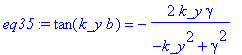
![]()
Taking into account:
| > | eq27; eq37 := n[cl]^2*k^2 - beta^2 = k_x^2 - gamma^2; eq27 - eq37; eq38 := gamma = sqrt( lhs(%) - k_y^2 ); |
![]()
![]()
![]()
![]()
we have:
| > | master[3] := subs(eq38,eq35); master[4] := subs(eq38,eq36); |
![master[3] := tan(k_y*b) = -2*k_y*(k^2*n[co]^2-k^2*n[cl]^2-k_y^2)^(1/2)/(-2*k_y^2+k^2*n[co]^2-k^2*n[cl]^2)](images/TFmodes228.gif)
![master[4] := tan(k_y*eta) = -(k^2*n[co]^2-k^2*n[cl]^2-k_y^2)^(1/2)/k_y](images/TFmodes229.gif)
![]() -modes
-modes
Now we shall make an analogous analysis for y-modes .
Within the core we have
| > | eq39 := e[z](x,y) = B*cos(k_x*(x+xi))*cos(k_y*(y+eta)); |
![]()
y-modes
correspond to
![]() . Hence,
. Hence,
| > | expand(-numer(rhs(f6))/I/beta) = 0; value(subs({eq39,omega=k/sqrt(epsilon0*mu0)},%)); dsolve(%,h[z](x,y)); |
,y)+1/beta*n^2*epsilon0*omega*diff(e[z](x,y),x) = 0](images/TFmodes233.gif)
,y)-1/beta*n^2*epsilon0*k/(epsilon0*mu0)^(1/2)*B*sin(k_x*(x+xi))*k_x*cos(k_y*(y+eta)) = 0](images/TFmodes234.gif)
 = 1/beta*n^2*epsilon0*k/(epsilon0*mu0)^(1/2)*B*sin(k_x*(x+xi))*k_x/k_y*sin(k_y*y+k_y*eta)+_F1(x)](images/TFmodes235.gif)
From the symmetry requirement we obtain:
| > | eq40 := h[z](x,y) = B*n^2*(k/beta)*(k_x/k_y)*sqrt(epsilon0/mu0)*sin(k_x*(x+xi))*sin(k_y*(y+eta)); |
 = B*n^2*k/beta*k_x/k_y*(epsilon0/mu0)^(1/2)*sin(k_x*(x+xi))*sin(k_y*(y+eta))](images/TFmodes236.gif)
The expressions for the longitudinal components result in those for the transverse fields:
| > | subs({eq39,eq40},f3): eq41 := simplify(%); subs({eq39,eq40},f4): eq42 := simplify(%); subs({eq39,eq40},f5): eq43 := simplify(%); |
![eq41 := e[x] = -I*B*sin(k_x*(x+xi))*k_x*cos(k_y*(y+eta))*(-beta^2+mu0*omega*n^2*k*(epsilon0/mu0)^(1/2))/U^2/beta](images/TFmodes237.gif)
![eq42 := e[y] = B*cos(k_x*(x+xi))*sin(k_y*(y+eta))*(beta^2*k_y^2+mu0*omega*n^2*k*k_x^2*(epsilon0/mu0)^(1/2))/U^2/beta/k_y*I](images/TFmodes238.gif)
![eq43 := h[x] = -I*B*n^2*cos(k_x*(x+xi))*sin(k_y*(y+eta))*(k*k_x^2*(epsilon0/mu0)^(1/2)+epsilon0*omega*k_y^2)/U^2/k_y](images/TFmodes239.gif)
| > | subs({k=omega*sqrt(epsilon0*mu0),U=sqrt(k_x^2+k_y^2)},eq43): simplify(%,radical,symbolic): eq44 := subs(omega=k/sqrt(epsilon0*mu0),%); subs(U=sqrt(-beta^2+k^2*n^2),eq42): simplify(%,radical,symbolic): eq45 := subs(omega=k/sqrt(epsilon0*mu0),%); subs(U=sqrt(-beta^2+k^2*n^2),eq41): simplify(%,radical,symbolic): eq46 := subs(omega=k/sqrt(epsilon0*mu0),%); |
![eq44 := h[x] = -I*epsilon0*k/(epsilon0*mu0)^(1/2)*sin(k_y*(y+eta))*cos(k_x*(x+xi))*n^2*B/k_y](images/TFmodes240.gif)
![eq45 := e[y] = B*cos(k_x*(x+xi))*sin(k_y*(y+eta))*(beta^2*k_y^2+k^2*n^2*k_x^2)/(-beta^2+k^2*n^2)/beta/k_y*I](images/TFmodes241.gif)
![]()
eq45 can be transformed by virtue of the following equalities:
| > | k_x^2 = n^2*k^2 - k_y^2 - beta^2; beta^2*k_y^2+k^2*n^2*k_x^2 = rhs(expand( %*k^2*n^2 )) + beta^2*k_y^2; factor(rhs(%)); U^2 = factor(n^2*k^2-beta^2); # Hence eq47 := e[y](x,y) = -B*cos(k_x*(x+xi))*sin(k_y*(y+eta))*(k^2*n^2-k_y^2)/beta/k_y*I; |
![]()
![]()
![]()
![]()
 = -I*B*cos(k_x*(x+xi))*sin(k_y*(y+eta))*(k^2*n^2-k_y^2)/beta/k_y](images/TFmodes247.gif)
| > | print(`Resulting system for core (n=n[co]):`); f30 := eq39; f31 := eq40; f32 := e[x](x,y) = rhs(eq46); f33 := h[x](x,y) = rhs(eq44); f34 := subs(k^2*n^2-k_y^2=k^2*n^2,eq47);# we use the smallness of k_y in comparison with k*n |
![]()
![]()
 = B*n^2*k/beta*k_x/k_y*(epsilon0/mu0)^(1/2)*sin(k_x*(x+xi))*sin(k_y*(y+eta))](images/TFmodes250.gif)
![]()
 = -I*epsilon0*k/(epsilon0*mu0)^(1/2)*sin(k_y*(y+eta))*cos(k_x*(x+xi))*n^2*B/k_y](images/TFmodes252.gif)
 = -I*B*cos(k_x*(x+xi))*sin(k_y*(y+eta))*k^2*n^2/beta/k_y](images/TFmodes253.gif)
If we consider only lower modes,
![]() vanishes (see above).
vanishes (see above).
For the lower air sector we have ( C and D are some constants):
| > | eq48 := C*cos(k_x*(xi-d))*cos(k_y*(y+eta))*exp(gamma*(x+d));# e[z] eq49 := D*cos(k_x*(xi-d))*sin(k_y*(y+eta))*exp(gamma*(x+d));# h[z] subs({e[z](x,y)=eq48,h[z](x,y)=eq49},rhs(f6)):# h[y] subs({omega=k/sqrt(epsilon0*mu0),n=n[cl]},numer(%)): simplify(%,radical,symbolic): numer(%); |
![]()
![]()
![]()
![]() =0 results in the condition:
=0 results in the condition:
| > | eq50 := beta*D*k_y*(epsilon0*mu0)^(1/2)+n[cl]^2*epsilon0*k*C*gamma = 0; |
![]()
Continuity of
![]() -component produces:
-component produces:
| > | value( subs({e[z](x,y) = eq48,h[z](x,y) = eq49},f4) ): subs(omega=k/sqrt(epsilon0*mu0),%): simplify( subs({U=sqrt(k_y^2-gamma^2),x=-d},rhs(%)) ) = subs({x=-d,n=n[co]},rhs(f34)); eq51 := %/cos(k_x*(-d+xi))/sin(k_y*(y+eta))/I; |
![-I*cos(k_x*(d-xi))*sin(k_y*(y+eta))*(beta*C*k_y*(epsilon0*mu0)^(1/2)+mu0*k*D*gamma)/(-k_y^2+gamma^2)/(epsilon0*mu0)^(1/2) = -I*B*cos(k_x*(-d+xi))*sin(k_y*(y+eta))*k^2*n[co]^2/beta/k_y](images/TFmodes261.gif)
![eq51 := -1/cos(k_x*(-d+xi))*cos(k_x*(d-xi))*(beta*C*k_y*(epsilon0*mu0)^(1/2)+mu0*k*D*gamma)/(-k_y^2+gamma^2)/(epsilon0*mu0)^(1/2) = -B*k^2*n[co]^2/beta/k_y](images/TFmodes262.gif)
| > | eq52 := C = solve(eq50,C); eq53 := simplify(lhs(subs(%,eq51))) = rhs(eq51); |
![eq52 := C = -beta*D*k_y*(epsilon0*mu0)^(1/2)/n[cl]^2/epsilon0/k/gamma](images/TFmodes263.gif)
![eq53 := -mu0*D*(-beta^2*k_y^2+k^2*n[cl]^2*gamma^2)/n[cl]^2/k/gamma/(-k_y^2+gamma^2)/(epsilon0*mu0)^(1/2) = -B*k^2*n[co]^2/beta/k_y](images/TFmodes264.gif)
As
| > | beta^2 = n[cl]^2*k^2 - k_y^2 + gamma^2; beta^2*k_y^2-k^2*n[cl]^2*gamma^2 = rhs(expand( %*k_y^2 )) - k^2*n[cl]^2*gamma^2; factor(rhs(%)); |
![]()
![]()
![]()
we have from eq53 :
| > | eq54 := D*sqrt(mu0/epsilon0)*k^2*n[cl]^2/(n[cl]^2*k*gamma) = rhs(eq53);# we use smallness of k_y in comparison with k*n |
![eq54 := D*(mu0/epsilon0)^(1/2)*k/gamma = -B*k^2*n[co]^2/beta/k_y](images/TFmodes268.gif)
| > | eq55 := D = solve(eq54,D); eq56 := simplify( subs(%,eq52),radical,symbolic ); |
![eq55 := D = -B*k*n[co]^2*gamma/(mu0/epsilon0)^(1/2)/beta/k_y](images/TFmodes269.gif)
![eq56 := C = B*n[co]^2/n[cl]^2](images/TFmodes270.gif)
So, we obtained the adjusting amplitudes for the longitudinal field-components.
| > | f35 := e[z](x,y) = subs(eq56,eq48); f36 := h[z](x,y) = subs(eq55,eq49); |
 = B*n[co]^2/n[cl]^2*cos(k_x*(-d+xi))*cos(k_y*(y+eta))*exp(gamma*(x+d))](images/TFmodes271.gif)
 = -B*k*n[co]^2*gamma/(mu0/epsilon0)^(1/2)/beta/k_y*cos(k_x*(-d+xi))*sin(k_y*(y+eta))*exp(gamma*(x+d))](images/TFmodes272.gif)
The transverse components result from the Maxwell's equations.
| > | subs({f35,f36},f3): eq57 := simplify(%); subs({f35,f36},f4): eq58 := simplify(%); subs({f35,f36},subs(n=n[cl],f5)): eq59 := simplify(%); |
![eq57 := e[x] = B*n[co]^2*cos(k_x*(d-xi))*cos(k_y*(y+eta))*gamma*exp(gamma*(x+d))*(-beta^2*(mu0/epsilon0)^(1/2)+mu0*omega*k*n[cl]^2)/U^2/n[cl]^2/(mu0/epsilon0)^(1/2)/beta*I](images/TFmodes273.gif)
![eq58 := e[y] = -I*B*n[co]^2*cos(k_x*(d-xi))*sin(k_y*(y+eta))*exp(gamma*(x+d))*(-beta^2*k_y^2*(mu0/epsilon0)^(1/2)+mu0*omega*k*gamma^2*n[cl]^2)/U^2/n[cl]^2/(mu0/epsilon0)^(1/2)/beta/k_y](images/TFmodes274.gif)
![eq59 := h[x] = B*n[co]^2*cos(k_x*(d-xi))*sin(k_y*(y+eta))*exp(gamma*(x+d))*(k*gamma^2-epsilon0*omega*k_y^2*(mu0/epsilon0)^(1/2))/U^2/(mu0/epsilon0)^(1/2)/k_y*I](images/TFmodes275.gif)
Hence
| > | subs({k=omega*sqrt(epsilon0*mu0),U=sqrt(k_y^2-gamma^2)},eq59): simplify(%,radical,symbolic): eq60 := subs(omega=k/sqrt(epsilon0*mu0),%); subs(U=sqrt(-gamma^2+k_y^2),eq58): simplify(%,radical,symbolic): eq61 := simplify( subs(omega=k/sqrt(epsilon0*mu0),%) ); subs(U=sqrt(-beta^2+k^2*n[cl]^2),eq57): simplify(%,radical,symbolic): eq62 := simplify( subs(omega=k/sqrt(epsilon0*mu0),%) ); |
![eq60 := h[x] = -I*epsilon0*k/(epsilon0*mu0)^(1/2)*exp(gamma*(x+d))*sin(k_y*(y+eta))*cos(k_x*(d-xi))*n[co]^2*B/k_y](images/TFmodes276.gif)
![eq61 := e[y] = B*n[co]^2*cos(k_x*(d-xi))*sin(k_y*(y+eta))*exp(gamma*(x+d))*(-beta^2*k_y^2+k^2*n[cl]^2*gamma^2)/(-k_y^2+gamma^2)/n[cl]^2/beta/k_y*I](images/TFmodes277.gif)
![eq62 := e[x] = B*n[co]^2*cos(k_x*(d-xi))*cos(k_y*(y+eta))*gamma*exp(gamma*(x+d))/n[cl]^2/beta*I](images/TFmodes278.gif)
As
| > | beta^2 = n[cl]^2*k^2 - k_y^2 + gamma^2; beta^2*k_y^2-gamma^2*k^2*n[cl]^2 = rhs( % )*k_y^2 - gamma^2*k^2*n[cl]^2; factor(rhs(%)); U^2 = factor(k_y^2-gamma^2); |
![]()
![]()
![]()
![]()
we have:
| > | f37 := e[y](x,y) = I*B*n[co]^2*(k^2/(beta*k_y))*cos(k_x*(-d+xi))*sin(k_y*(y+eta))*exp(gamma*(x+d)); f38 := e[x](x,y) = rhs(eq62); f39 := h[x](x,y) = rhs(eq60); |
 = B*n[co]^2*k^2/beta/k_y*cos(k_x*(-d+xi))*sin(k_y*(y+eta))*exp(gamma*(x+d))*I](images/TFmodes283.gif)
 = B*n[co]^2*cos(k_x*(d-xi))*cos(k_y*(y+eta))*gamma*exp(gamma*(x+d))/n[cl]^2/beta*I](images/TFmodes284.gif)
 = -I*epsilon0*k/(epsilon0*mu0)^(1/2)*exp(gamma*(x+d))*sin(k_y*(y+eta))*cos(k_x*(d-xi))*n[co]^2*B/k_y](images/TFmodes285.gif)
| > | print(`Resulting system for lower air sector (n=n[cl]):`); f35; f36; f38; f37; f39; |
![]()
 = B*n[co]^2/n[cl]^2*cos(k_x*(-d+xi))*cos(k_y*(y+eta))*exp(gamma*(x+d))](images/TFmodes287.gif)
 = -B*k*n[co]^2*gamma/(mu0/epsilon0)^(1/2)/beta/k_y*cos(k_x*(-d+xi))*sin(k_y*(y+eta))*exp(gamma*(x+d))](images/TFmodes288.gif)
 = B*n[co]^2*cos(k_x*(d-xi))*cos(k_y*(y+eta))*gamma*exp(gamma*(x+d))/n[cl]^2/beta*I](images/TFmodes289.gif)
 = B*n[co]^2*k^2/beta/k_y*cos(k_x*(-d+xi))*sin(k_y*(y+eta))*exp(gamma*(x+d))*I](images/TFmodes290.gif)
 = -I*epsilon0*k/(epsilon0*mu0)^(1/2)*exp(gamma*(x+d))*sin(k_y*(y+eta))*cos(k_x*(d-xi))*n[co]^2*B/k_y](images/TFmodes291.gif)
For the upper air sector (due to the coordinate shift and the change of the
![]() -sign) we have:
-sign) we have:
| > | print(`Resulting system for upper air sector (n=n[cl]):`); f40 := subs({d=0,gamma=-gamma},f35); f41 := subs({d=0,gamma=-gamma},f36); f42 := subs({d=0,gamma=-gamma},f38); f43 := subs({d=0,gamma=-gamma},f37); f44 := subs({d=0,gamma=-gamma},f39); |
![]()
 = B*n[co]^2/n[cl]^2*cos(k_x*xi)*cos(k_y*(y+eta))*exp(-gamma*x)](images/TFmodes294.gif)
 = B*k*n[co]^2*gamma/(mu0/epsilon0)^(1/2)/beta/k_y*cos(k_x*xi)*sin(k_y*(y+eta))*exp(-gamma*x)](images/TFmodes295.gif)
 = -I*B*n[co]^2*cos(-k_x*xi)*cos(k_y*(y+eta))*gamma*exp(-gamma*x)/n[cl]^2/beta](images/TFmodes296.gif)
 = B*n[co]^2*k^2/beta/k_y*cos(k_x*xi)*sin(k_y*(y+eta))*exp(-gamma*x)*I](images/TFmodes297.gif)
 = -I*epsilon0*k/(epsilon0*mu0)^(1/2)*exp(-gamma*x)*sin(k_y*(y+eta))*cos(-k_x*xi)*n[co]^2*B/k_y](images/TFmodes298.gif)
Now we turn to the right air sector. We shall use the condition of
![]() .
.
| > | eq61 := B*cos(k_x*(x+xi))*cos(k_y*(b+eta))*exp(-gamma*(y-b));# e[z] eq62 := C*sin(k_x*(x+xi))*cos(k_y*(b+eta))*exp(-gamma*(y-b));# h[z] subs({e[z](x,y)=eq61,h[z](x,y)=eq62},rhs(f6)):# h[y] subs({omega=k/sqrt(epsilon0*mu0),n=n[cl]},numer(%)): simplify(%,radical,symbolic): numer(%); |
![]()
![]()
![]()
| > | eq63 := beta*C*gamma*(epsilon0*mu0)^(1/2)+n[cl]^2*epsilon0*k*B*k_x = 0; eq64 := C = solve(%,C); |
![]()
![eq64 := C = -n[cl]^2*epsilon0*k*B*k_x/beta/gamma/(epsilon0*mu0)^(1/2)](images/TFmodes304.gif)
| > | f45 := e[z](x,y) = eq61; f46 := h[z](x,y) = subs(eq64,eq62); |
![]()
 = -n[cl]^2*epsilon0*k*B*k_x/beta/gamma/(epsilon0*mu0)^(1/2)*sin(k_x*(x+xi))*cos(k_y*(b+eta))*exp(-gamma*(y-b))](images/TFmodes306.gif)
Hence we can obtain the remaining field-components:
| > | subs({f45,f46},f3): eq65 := simplify(%); subs({f45,f46},f4): eq66 := simplify(%); subs({f45,f46},subs(n=n[cl],f5)): eq67 := simplify(%); |
![eq65 := e[x] = B*sin(k_x*(x+xi))*k_x*cos(k_y*(b+eta))*exp(-gamma*(y-b))*(beta^2*(epsilon0*mu0)^(1/2)-mu0*omega*k*n[cl]^2*epsilon0)/U^2/beta/(epsilon0*mu0)^(1/2)*I](images/TFmodes307.gif)
![eq66 := e[y] = B*cos(k_x*(x+xi))*cos(k_y*(b+eta))*exp(-gamma*(y-b))*(beta^2*gamma^2*(epsilon0*mu0)^(1/2)-mu0*omega*n[cl]^2*epsilon0*k*k_x^2)/U^2/beta/gamma/(epsilon0*mu0)^(1/2)*I](images/TFmodes308.gif)
![eq67 := h[x] = -I*n[cl]^2*epsilon0*B*cos(k_x*(x+xi))*cos(k_y*(b+eta))*exp(-gamma*(y-b))*(-k*k_x^2+omega*(epsilon0*mu0)^(1/2)*gamma^2)/U^2/gamma/(epsilon0*mu0)^(1/2)](images/TFmodes309.gif)
| > | subs({k=omega*sqrt(epsilon0*mu0),U=sqrt(n[cl]^2*k^2-beta^2)},eq65): simplify(%,radical,symbolic): eq60 := subs(omega=k/sqrt(epsilon0*mu0),%); subs(U=sqrt(n[cl]^2*k^2-beta^2),eq66): simplify(%,radical,symbolic): eq61 := simplify( subs(omega=k/sqrt(epsilon0*mu0),%) ); subs(U=sqrt(k_x^2-gamma^2),eq67): simplify(%,radical,symbolic): eq62 := simplify( subs(omega=k/sqrt(epsilon0*mu0),%) ); |
![eq60 := e[x] = -I*B*sin(k_x*(x+xi))*k_x*cos(k_y*(b+eta))*exp((-y+b)*gamma)/beta](images/TFmodes310.gif)
![eq61 := e[y] = -I*B*cos(k_x*(x+xi))*cos(k_y*(b+eta))*exp(-gamma*(y-b))*(-beta^2*gamma^2+k^2*n[cl]^2*k_x^2)/(k^2*n[cl]^2-beta^2)/beta/gamma](images/TFmodes311.gif)
![eq62 := h[x] = n[cl]^2*epsilon0*B*cos(k_x*(x+xi))*cos(k_y*(b+eta))*exp(-gamma*(y-b))*k/gamma/(epsilon0*mu0)^(1/2)*I](images/TFmodes312.gif)
As
| > | k_x^2 = n[cl]^2*k^2 + gamma^2 - beta^2; -beta^2*gamma^2+k_x^2*k^2*n[cl]^2 = rhs( % )*k^2*n[cl]^2 - gamma^2*beta^2; factor(rhs(%)); U^2 = factor(k^2*n[cl]^2-beta^2); |
![]()
![]()
![]()
![]()
we have:
| > | f47 := e[x](x,y) = rhs(eq60)*(k^2*n[cl]^2-beta^2)/(beta^2-k^2*n[cl]^2); f48 := h[x](x,y) = rhs(eq62); f49 := e[y](x,y) = -I*B*(k^2*n[cl]^2+gamma^2)/(beta*gamma)*cos(k_x*(x+xi))*cos(k_y*(b+eta))*exp(-gamma*(y-b)); |
 = -I*B*sin(k_x*(x+xi))*k_x*cos(k_y*(b+eta))*exp((-y+b)*gamma)/beta*(k^2*n[cl]^2-beta^2)/(beta^2-k^2*n[cl]^2)](images/TFmodes317.gif)
 = n[cl]^2*epsilon0*B*cos(k_x*(x+xi))*cos(k_y*(b+eta))*exp(-gamma*(y-b))*k/gamma/(epsilon0*mu0)^(1/2)*I](images/TFmodes318.gif)
 = -I*B*(k^2*n[cl]^2+gamma^2)/beta/gamma*cos(k_x*(x+xi))*cos(k_y*(b+eta))*exp(-gamma*(y-b))](images/TFmodes319.gif)
| > | print(`Resulting system for right air sector (n=n[cl]):`); f45; f46; f47; f48; f49; |
![]()
![]()
 = -n[cl]^2*epsilon0*k*B*k_x/beta/gamma/(epsilon0*mu0)^(1/2)*sin(k_x*(x+xi))*cos(k_y*(b+eta))*exp(-gamma*(y-b))](images/TFmodes322.gif)
 = -I*B*sin(k_x*(x+xi))*k_x*cos(k_y*(b+eta))*exp((-y+b)*gamma)/beta*(k^2*n[cl]^2-beta^2)/(beta^2-k^2*n[cl]^2)](images/TFmodes323.gif)
 = n[cl]^2*epsilon0*B*cos(k_x*(x+xi))*cos(k_y*(b+eta))*exp(-gamma*(y-b))*k/gamma/(epsilon0*mu0)^(1/2)*I](images/TFmodes324.gif)
 = -I*B*(k^2*n[cl]^2+gamma^2)/beta/gamma*cos(k_x*(x+xi))*cos(k_y*(b+eta))*exp(-gamma*(y-b))](images/TFmodes325.gif)
The coordinate shift and the change of the
![]() -sign produce:
-sign produce:
| > | print(`Resulting system for left air sector (n=n[cl]):`); f50 := subs({b=0,gamma=-gamma},f45); f51 := subs({b=0,gamma=-gamma},f46); f52 := subs({b=0,gamma=-gamma},f47); f53 := subs({b=0,gamma=-gamma},f48); f54 := subs({b=0,gamma=-gamma},f49); |
![]()
![]()
 = n[cl]^2*epsilon0*k*B*k_x/beta/gamma/(epsilon0*mu0)^(1/2)*sin(k_x*(x+xi))*cos(k_y*eta)*exp(gamma*y)](images/TFmodes329.gif)
 = -I*B*sin(k_x*(x+xi))*k_x*cos(k_y*eta)*exp(gamma*y)/beta*(k^2*n[cl]^2-beta^2)/(beta^2-k^2*n[cl]^2)](images/TFmodes330.gif)
 = -I*n[cl]^2*epsilon0*B*cos(k_x*(x+xi))*cos(k_y*eta)*exp(gamma*y)*k/gamma/(epsilon0*mu0)^(1/2)](images/TFmodes331.gif)
 = B*(k^2*n[cl]^2+gamma^2)/beta/gamma*cos(k_x*(x+xi))*cos(k_y*eta)*exp(gamma*y)*I](images/TFmodes332.gif)
Again, the requirement of the
![]() -continuity on the horizontal interfaces leads to
-continuity on the horizontal interfaces leads to
| > | subs({n=n[co],x=-d},rhs(f31)) - subs(x=-d,rhs(f36)):# lower interface eq63 := numer(simplify(%,radical,symbolic))/B/k/n[co]^2/sin(k_y*(y+eta))/epsilon0 = 0; subs({n=n[co],x=0},rhs(f31)) - subs(x=0,rhs(f41)):# upper interface eq64 := numer(simplify(%,radical,symbolic))/B/k/n[co]^2/sin(k_y*(y+eta))/epsilon0 = 0; |
![]()
![]()
As it was above, let us consider this system in the following way:
| > | subs({cos(k_x*xi)=X,sin(k_x*xi)=Y},expand(lhs(eq63))): eq65 := collect(%,{X,Y}); eq66 := collect(subs({cos(k_x*xi)=X,sin(k_x*xi)=Y},lhs(eq64)),{X,Y}); |
![]()
![]()
The solution exists if the determinant of this system is equal to zero:
| > | matrix(2,2,[coeff(eq65,X),coeff(eq65,Y),coeff(eq66,X),coeff(eq66,Y)]); det(%) = 0; eq67 := collect(%,{sin(k_x*d),cos(k_x*d)}); |
![matrix([[-k_x*sin(k_x*d)+gamma*cos(k_x*d), k_x*cos(k_x*d)+gamma*sin(k_x*d)], [-gamma, k_x]])](images/TFmodes338.gif)
![]()
![]()
Hence
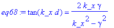
| > | eq68 := tan(k_x*d) = 2*k_x*gamma/(k_x^2-gamma^2); eq69 := tan(k_x*xi) = gamma/k_x; |
![]()
By virtue of
| > | eq29; |
![]()
we obtain the equations for
![]() and
and
![]() :
:
| > | master[5] := subs(eq29,eq68); master[6] := subs(eq29,eq69); |
![master[5] := tan(k_x*d) = 2*k_x*(k^2*n[co]^2-k^2*n[cl]^2-k_x^2)^(1/2)/(2*k_x^2-k^2*n[co]^2+k^2*n[cl]^2)](images/TFmodes346.gif)
![master[6] := tan(k_x*xi) = (k^2*n[co]^2-k^2*n[cl]^2-k_x^2)^(1/2)/k_x](images/TFmodes347.gif)
The continuity conditions for the vertical interfaces result in:
| > | subs({n=n[co],y=b},rhs(f31)) - subs(y=b,rhs(f46)):# right interface eq70 := numer(simplify(%,radical,symbolic))/B/k/k_x/sin(k_x*(x+xi))/epsilon0 = 0; subs({n=n[co],y=0},rhs(f31)) - subs(y=0,rhs(f51)):# left interface eq71 := numer(simplify(%,radical,symbolic))/B/k/k_x/sin(k_x*(x+xi))/epsilon0 = 0; |
![]()
![]()
| > | subs({cos(k_y*eta)=X,sin(k_y*eta)=Y},expand(lhs(eq70))): eq72 := collect(%,{X,Y}); eq73 := collect(subs({cos(k_y*eta)=X,sin(k_y*eta)=Y},lhs(eq71)),{X,Y}); |
![]()
![]()
| > | matrix(2,2,[coeff(eq72,X),coeff(eq72,Y),coeff(eq73,X),coeff(eq73,Y)]); det(%) = 0; eq74 := collect(%,{sin(k_y*b),cos(k_y*b)});; |
![matrix([[n[co]^2*gamma*sin(k_y*b)+n[cl]^2*k_y*cos(k_y*b), n[co]^2*gamma*cos(k_y*b)-n[cl]^2*k_y*sin(k_y*b)], [-n[cl]^2*k_y, n[co]^2*gamma]])](images/TFmodes352.gif)
![]()
![]()
Hence
| > | eq75 := tan(k_y*b) = 2*n[co]^2*n[cl]^2*gamma*k_y/(n[cl]^4*k_y^2-n[co]^4*gamma^2); eq76 := tan(k_y*eta) = n[cl]^2*k_y/(n[co]^2*gamma); |
![eq75 := tan(k_y*b) = 2*n[co]^2*n[cl]^2*gamma*k_y/(n[cl]^4*k_y^2-n[co]^4*gamma^2)](images/TFmodes355.gif)
![eq76 := tan(k_y*eta) = n[cl]^2*k_y/n[co]^2/gamma](images/TFmodes356.gif)
| > | master[7] := subs(eq38,eq75); master[8] := subs(eq38,eq76); |
![master[7] := tan(k_y*b) = 2*n[co]^2*n[cl]^2*(k^2*n[co]^2-k^2*n[cl]^2-k_y^2)^(1/2)*k_y/(n[cl]^4*k_y^2-n[co]^4*(k^2*n[co]^2-k^2*n[cl]^2-k_y^2))](images/TFmodes357.gif)
![master[8] := tan(k_y*eta) = n[cl]^2*k_y/n[co]^2/(k^2*n[co]^2-k^2*n[cl]^2-k_y^2)^(1/2)](images/TFmodes358.gif)
| > |
The equations
master1, master3
and
master5, master7
can be solved by Matlab-procedures (files
f2.m, f3.m, f4.m, f5.m and
tap_f2.m, tap_f3.m). The basic functions are
tap_f2
(x
)
and
tap_f3
(x
)
whose arguments are the mode indexes
p
and
q
giving the root's order (the mode's order, as well). The result are the effective refractive indexes for the x- and y-modes in the spectral range of 0.65 - 3
![]() m (we supposed that the fiber's material is the SF6 glass). The obtained results are written in the files
neff2.dat
and
neff3.dat
(the fiber diameter dimension is 4.46 x 3.61
m (we supposed that the fiber's material is the SF6 glass). The obtained results are written in the files
neff2.dat
and
neff3.dat
(the fiber diameter dimension is 4.46 x 3.61
![]() m). The effective refractive index and its fitting are shown below for the
m). The effective refractive index and its fitting are shown below for the
![]() and
and
![]() modes.
modes.
| > | # Ex-mode neff2 := readdata(`neff2.dat`,2,float): for i from 1 to 301 do Q2[i] := [neff2[i,1],neff2[i,2]]: od: p1 := statplots[scatterplot]([Q2[k][1] $k=1..301],[Q2[k][2] $k=1..301]): eq77 := fit[leastsquare[[x,y], y=a0+a1*x^2+a2/x^2+a3/x^4+a4/x^6+a5/x^8+a7/x+a8*x+a9*x^3+a10/x^3+a11*x^9+a12/x^9+a13*x^10+a14*x^11+a15/x^10+a16/x^11,{a0,a1,a2,a3,a4,a5,a6,a7,a8,a9,a10,a11,a12,a13,a14,a15,a16}]]([[Q2[k][1] $k=1..301],[Q2[k][2] $k=1..301]]): p2 := plot(rhs(eq77),x=0.65..3,color=red): # Ey-mode neff3 := readdata(`neff3.dat`,2,float): for i from 1 to 301 do Q3[i] := [neff3[i,1],neff3[i,2]]: od: p3 := statplots[scatterplot]([Q3[k][1] $k=1..301],[Q3[k][2] $k=1..301]): eq78 := fit[leastsquare[[x,y], y=a0+a1*x^2+a2/x^2+a3/x^4+a4/x^6+a5/x^8+a7/x+a8*x+a9*x^3+a10/x^3+a11*x^9+a12/x^9+a13*x^10+a14*x^11+a15/x^10+a16/x^11,{a0,a1,a2,a3,a4,a5,a6,a7,a8,a9,a10,a11,a12,a13,a14,a15,a16}]]([[Q3[k][1] $k=1..301],[Q3[k][2] $k=1..301]]): p4 := plot(rhs(eq78),x=0.65..3,color=blue): display(p1,p2,p3,p4,axes=boxed,title=`refractive index vs. wavelength (in mkm)`); |
![[Maple Plot]](images/TFmodes363.gif)
As it was shown above, even for the rectangular core we have to make some assumptions, which don't allow considering the higher-order modes. When the fiber core has a very complicated shape (as in the case of the so-called photonic-crystal fibers), the analytical treatment is not possible at all and we have to use the numerical solution of the Helmholtz's equations in the conditions of the complicated geometry. The possible way is to use FEMLAB 2.2 package based on MATLAB. Electromagnetic module of this package's version allows the solution of the harmonically time dependent Maxwell's equations for the longitudinal field components of the hybrid fiber modes:
![[Maple Bitmap]](images/TFmodes364.gif)
(see User Guide). The geometry can be extracted from the micrography of the real fiber (by means of MATLAB Image Processing Toolbox, for example). Since, the unknown effective refractive index defines both the phase velocity
![]() and the eigenvalue
and the eigenvalue
![]() , we need the iteration procedure to obtain it. Note, that the presence of the spurious modes in the case of the complicated geometries requires the visual control of the energy and field distributions for the obtained solutions.
, we need the iteration procedure to obtain it. Note, that the presence of the spurious modes in the case of the complicated geometries requires the visual control of the energy and field distributions for the obtained solutions.
V.L.Kalashnikov, Wien 18.12.2003