The occurrence of PDE's in Physics follows from the application of conservation laws in almost all areas (See Potter). For example, consider the principle of conservation of electric charge. In any volume v containing mobile charges the rate of change of total charge must be equal to the current flowing through its bounding surface. Expressed as an equation
![]()
The minus sign comes because ds is the outward normal.
Applying Gauss's divergence theorem (surface integral of normal component equals volume integral of divergence) leads to
![]()
which allows us to express the equation in the form
![]()
and hence, since
![]()
we have
![]()
because (div.curl. anyvector=0), we can write the expression in brackets as the curl of something, here the something being the magnetic intensity
![]()
thus deriving one of the Maxwell's equations. Similarly, we can derive
![]()
from the principle of conservation of magnetic flux, the diffusion equation from principle of conservation of energy, and the fluid equation of motion from the principle of conservation of mass and momentum.
The PDE is universal. Since many important physical systems defy analytical treatment the methods of solving PDE's computationally become very important.
![]()
If the equation is separable, the second term is absent. a, b, c, d, e, f, g, are coefficients which may be constant, dependent on x and y and (horrors!) possibly on u also, in which case the PDE becomes a non-linear nightmare.
The first step towards simplification is the creation of categories depending on the relative magnitudes of the coefficients. The equation is called elliptic, parabolic or hyperbolic depending on whether

respectively .
These names follow from the characteristic curves of the equations (see Smith, Sen and Krishnamurthi). It can be shown that at every point in the x-y plane there are two directions along which the partial derivatives vanish and the PDE is reduced to an ordinary differential equation. The existence of these curves is important in solving hyperbolic PDEs in a method known as the method of characteristics.
There is another classification which is more interesting to the physicist. The parabolic and hyperbolic PDEs are more often found to describe time dependent initial value problems, in which the starting configuration of the physical system at time t=0 is known and one wishes to find out the how it evolves with time. The elliptic PDE describes static problems, where the distribution of some quantity over space is required to be found at a given time, with the values of the quantity at the boundaries of the region being known.
The following are taken to be the prototype equations for each class:
Hyperbolic PDE: The wave equation:![]()
Parabolic PDE; The diffusion equation: ![]()
Elliptic PDE: Poissons equation: ![]()
It can also be seen that the elliptic PDE follows from the other two when the time derivatives go to zero, presumably when t tends to infinity and the solution reaches a steady state.
A decision tree to locate a suitable method of solving PDEs is given
in Hockney and Eastwood. Basically the technique is to use mesh relaxation
or a matrix method for nonseparable forms, or one of the so called Direct
methods (Fourier, cyclic reduction) if the PDE is separable on a rectangular
geometry with constant coefficients and periodic boundary conditions. There
is a class of methods known as Multigrid which are an extension of mesh
relaxation but more
widely applicable than direct methods and are as fast in comparison.
We will be discussing relaxation methods in particular, because they
are widely applicable to many types of problems, and easy to program, though
not as efficient as multi-grid methods, which we will discuss only qualitatively.
Though we will take up only elliptic PDEs the methods are applicable to
hyperbolic and parabolic PDEs as well. The Poisson equation in 2-D will
be used as the prototype where the source term, would represent charge
density in a
physical situation involving charges, or mass density in gravitational
phenomena; u then represents the appropriate electrostatic or gravitational
potential, respectively.

where  is the separation between points,
assumed to be the same along x and y. The values of the source term are
known on these points. The values of u are to be found. Using Taylor's
expansion about each point it is easy to get the standard five point formula
for the Poisson equation as:
is the separation between points,
assumed to be the same along x and y. The values of the source term are
known on these points. The values of u are to be found. Using Taylor's
expansion about each point it is easy to get the standard five point formula
for the Poisson equation as:
![]()
This is the finite difference representation of Poissons equation in 2-D in cartesian coordinates. Since we are interested in a finite region, we should know the values of u on the boundaries of this region. These values themselves can be specified at each point on the boundary (Dirichlet boundary conditions)or the normal derivatives of these values may be specified (Neumann boundary conditions), or a mixture (mixed boundary conditions, but not both on the same point).
We can represent the above finite difference equation (FDE) in matrix notation as follows after pulling all the known boundary points to the right hand side:
Au =b
The matrix of coefficients, A, is tridiagonal, and the unknown values u are expressed as a column vector .Standard methods of solving a system of linear equations are all applicable here, and techniques like Gauss elimination, LU decomposition, etc., are well known (see for example Sen and Krishnamurthi and Teukolsky, et al).
The general second order PDE will have a similar form when discretised, but the non-zero values will not be constants as in this case.
Consider the parabolic PDE in 2-D:
![]()
The difference form of this is
![]()
where n represents the timelevel.
Difference equations similar to the above are used in iteratively solving the diffusion equation itself. In our case if we set the timestep to be
![]()
then we have
![]()
Thus we can get a new value of u at step (n+1) using the four surrounding old values at step n and the source term. The procedure is to sweep through the points starting from one comer row by row and calculate a new value for u using the formula above at each point. This is repeated till some predeterminimaed accuracy is attained.
This is called the Jacobi method, and is the standard with which all the other relaxation methods are compared. A simple improvement to this results in the Gauss-Seidel (G-S) method, in which the new values of u are used in the formula above as soon as they are available, that is, the points which are already updated (to the left and top of the current point, if we start from the top left corner of the mesh) are used immediately in calculate the new value of u for the current point. This results in the formula
![]()
The Jacobi method is also called simultaneous displacement, because the new ones simultaneously replace the all the old values in the column vector u, whereas the G-S method is called the successive displacement.
We can split the coefficient matrix A into parts, an upper and a lower triangular matrix with all diagonal elements zero, and a diagonal matrix which here is just the Identity matrix. Hence
![]()
where b represents the source terms and the known values at the boundary
.This can be expressed as
![]()
The Jacobi iteration is thus
![]()
and the G-S iteration is
![]()
which can be written as
![]()
The rate of convergence of the relaxation method depends on how fast the error, which is the difference between the true and approximate solutions, reduces as the number of iterations increase. The error vector at any time is given by the difference between the true solution u and the actual vector at the current stage n
![]()
Hence for the Jacobi iteration the error vector changes as
![]()
while for the G-S it moves as
![]()
In the above the coefficient of the RHS is the same matrix that is used in the iteration and is called the iteration matrix. Because this remains the same throughout, the iterative process is called stationary. If the iteration matrix is denoted by H then
![]()
Let H have the set of linearly independent eigenvectors v; with eigenvalues
l so that ![]() can be expressed
as
can be expressed
as
![]()
Hence ![]() is
is
![]()
and consequently
![]()
This means that e^n decreases with n only if all |l[s]| are less than
1. The largest value of |l[s]| is called the spectral radius of H, denoted
by  . For large values of n, the decrease
in e will be governed by
. For large values of n, the decrease
in e will be governed by ![]() ,
and
,
and ![]() is defined to be the
asymptotic rate of convergence. It can be shown (see Smith) that for the
Jacobi Iteration matrix the spectral radius is
is defined to be the
asymptotic rate of convergence. It can be shown (see Smith) that for the
Jacobi Iteration matrix the spectral radius is
![]()
for a JxL rectangular mesh. Hence decreasing the mesh width to get a more accurate solution will lead to larger number of iterations due to the increase in the values of J and L. In general, the number of iterations are proportional to JxL.
It can also be shown that the spectral radius of the G-S iteration matrix is the square of the spectral radius of the Jacobi iteration matrix, hence the rate of convergence of the G-S method is double that of the Jacobi method.
For regular solutions of large size problems (where meshes exceed 100x100), these rates are too slow and these methods are not used unless the solution is required only for a few cases.
A significant increase in the convergence rate and decrease in the number of iterations follows from the fact that the new values of u which are calculated at each point may be pushed closer to the final solution by adding to each one a small increment proportional to the change which has taken place. This is known as successive over- relaxation, or the SOR method.
The iteration in this method is obtained from the G-S iteration
![]()
by solving for u(n+1) and adding and subtracting u(n) on the RHS. We get
![]()
It can be seen that the last tem1 in the RHS (in square brackets) is the difference between the current value and the new value of u at step n. This is called the residual which, if denoted by R, we can write
![]()
In the SOR method we push the residual in the direction of the change
by a factor  to get the iteration
![]()
The pitfall to avoid is not to make a correction that is too large,
or the value of u may cross the solution at some stage and start oscillating.
It can be shown that there is an optimum value of  by which this push should be made, given by
where  is the spectral radius of the Jacobi
iteration matrix (L+U). If
is the spectral radius of the Jacobi
iteration matrix (L+U). If  lies between
0 and 2 the iteration converges. If
lies between
0 and 2 the iteration converges. If  is between
1 and 2 the convergence is faster than the G-S method, under certain conditions
commonly prevalent.
is between
1 and 2 the convergence is faster than the G-S method, under certain conditions
commonly prevalent.
The rate of convergence using SOR is strongly dependent on the value
of  . If the optimum value is used then the
spectral radius for the SOR is given by
. If the optimum value is used then the
spectral radius for the SOR is given by
In general the number of iterations required is proportional to the
number of points along one side of the mesh, hence this method leads to
a significant saving in time as compared to G-S or Jacobi methods.
The convergence rate in SOR and G-S (and therefore the number of iterations)
is also dependent upon the order in which the mesh points are scanned,
since the latest values in iteration (n+1) are used to calculate other
values in the same iteration. In the Jacobi method, however, this is not
the case because the (n+1)th iteration employs points only from the n-th
iteration.
The straightforward method is to start at one corner and proceed along the rows. Another method follows from the fact that if we consider the points to be coloured alternately black and white as on a chessboard, then during each iteration the black points are evaluated using only the white points and vice-versa. It is thus possible to iterate over one set of points, (called a half-iteration), and then over the other set. This method is referred to as white-black, (sometimes red-black) or odd-even ordering, where odd or even refers to the sum of the indices (j+i) for the mesh point.
The optimum value  is the asymptotic optimum,
and thus is the proper value only after a lage number of iterations are
already over. It would not be a good initial choice. A method known as
Chebyshev acceleration uses the white-black ordering to adjust
from an initial value of 1, at each half iteration according to the formulae
is the asymptotic optimum,
and thus is the proper value only after a lage number of iterations are
already over. It would not be a good initial choice. A method known as
Chebyshev acceleration uses the white-black ordering to adjust
from an initial value of 1, at each half iteration according to the formulae
Its value quickly reaches the optimum value as n increases. This results in a lesser total number of iterations as compared to the SOR, even though the asymptotic rate of convergence is the same.
For illustration consider a PDE in 1-D whose solution is analytically available. We try to find the solution by iterating over points along a line with boundary conditions being specified at the end points. We can monitor the error at each mesh point at different stages, since the actual solution is known in advance. A plot of the error versus position will define a curve that changes as the iteration progresses. If we carry out a fourier analysis of this curve at different iterations, we will find that the high frequency components reduce rapidly and much faster than the low frequency components.
The finite difference equation is thus a very good smoothing operator. If the iteration could be adjusted to reduce the low frequency components equally fast, then the number of iterations would be considerably reduced. Since the number of frequency components are ultimately dependent on the mesh size, we can first do some iterations on a fine mesh to reduce the high frequency components, then interpolate the approximate solution to a coarse mesh defined over the same region, iterate to reduce the low frequency components, then interpolate back to the fine mesh for more iterations to get the final solution. The movement from fine to coarse and back (a cycle) can be extended over several levels of different mesh sizes. Hence the name Multi-Grid. At each level a few cycles are performed before moving on to the next level.
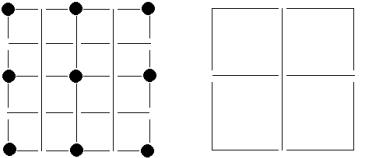
Consider two grids in 2-D. The coarse grid has a mesh size twice that
of the fine grid. lt can be seen that during the interpolation of mesh
values from one grid to the other, a mesh point in the coarse grid will
receive contributions from the one point which coincides with its position
plus eight other mesh points belonging to the fine grid. In the reverse
direction, a mesh point
belonging to the fine grid will either be surrounded by four coarse
mesh points, or lie between two of them (see figure below). Hence the interpolation
of values from the coarse mesh to the fine mesh will be different. The
fine to coarse interpolation is called restriction, and the opposite interpolation
is called prolongation.
In the figure below the points shown as full circles are common to both the fine and coarse grids.
A direct representation of the restriction and prolongation operators is to show, by means of a matrix, the fraction of the value of the coarse mesh point that is allotted to the nine fine mesh points, or taken from them. A widely followed scheme is bilinear interpolation (which is commonly used in fluid and particle simulations also). In this case the prolongation operator is denoted by the symbol:
 (Coarse to Fine)
This shows that half the value goes to each of the four nearest-neighbours, a quarter each to the four next nearest, and the full value is retained on the point which coincides with it.
The restriction operator has the symbol:
 (Fine to Coarse)
This shows that the coarse mesh point receives a sixteenth part of the value of each of the four next nearest neighbours, one-eighth of each of the nearest-neighbours, and one fourth of the mesh point which coincides with it. This totals to unity. Other weighing scheme may also be used, and the symbol will obviously depend on the mesh widths of the fine and coarse grids.
The full multi-grid method starts with the exact solution of the finite difference equations on a very coarse grid and successively reduces the mesh size, carrying out one or more two-grid cycles at each level before going to the finer grid of the next higher level. This process is repeated until the solution is reached to the desired accuracy. For more details see Hackbusch, which contains a large bibliography, and Teukolsky, et al.
Hackbusch, W., Multi-Grid methods and Applications, Springer series in Computational Mathematics No 4, Springer-Verlag, 1985
Hockney, R.W., Eastwood, J.E., Computer Simulation using Particles, McGraw-Hill, 1987
MacKeown, P.K., Newman, D.J., Computational Techniques in Physics, Adam Hilger, 1987
Potter, D.E., "Occurrence of Partial Differential Equations in Physics and the mathematical nature of equations", Computing as a Language of Physics, IAEA, 1972
Press, W.H., Teukolsky, S.A., Vetterling, W.T., Flannery, B.P., Numerical Recipes-The Art of Scientific Computing, 2nd edition, Cambridge University Press, 1992, Indian reprint by Foundation Books, N.Delhi, 1993
Smith. G.D., Numerical solution to Partial Differential Equations, Oxford University Press
Sen, S.K., Krishnamurthy, E.V., Computer-based Numerical Algorithms, Affiliated East-West Press
Last updated: 1 May, 2004
Copyright (c) 2000-2004
Kartik Patel