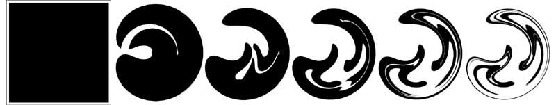
Figure 5: Five recursive applications of [Polar > Rotate 90 degrees > Polar > Rotate -90 degrees] to a square.
Creating Images of ICTS
Images of ICTS can be created in several different ways, each
highlighting a different aspect of the contortions of the plane caused by these
repeated transformations.
One of the simplest methods is illustrated in Figure 5. This images was created
starting from a square filled with black points. As the ICTS is applied to the
data the original square is converted into an appoximation of the shape of this
ICTS's attactor.
Figure 5: Five recursive applications of [Polar > Rotate 90 degrees >
Polar > Rotate -90 degrees] to a square.
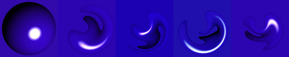
Figure
6: Transformations of an image of a sphere.
A second method of illustrating ICTS, which allows many of the stages of transformation to be seen together, is to start with a collection of distinct horizontal lines. The image after each complete iteration of the transformation sequence is then overlayed. Since most of the ICTS discussed here are 'contractive' (the area covered by the original data set shrinks with each application of the transformation sequence), and the stages in the squence of images are overlapping; having sparse coverage of the original plane allows each stage to be glimsed. The density of these lines should be lower for ICTS that contract more slowly. An example of this method is shown in Figure 7.
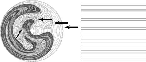
Figure 7: Horizontal lines transformed by [Polar > Rotate 90 degrees >
Polar > Flip Horizontal].
The arrows highlight the copies of the horizintal lines as they look after each
pair of elementary transformation steps.
Another method for generating esthecally pleasing images of ICTS is to apply the transformation to a solid square as in Figure 5, but rather than use a completely solid color use a mostly translucent or light grey. Layering the resultant stages of transformation creates a greyscale topographic map of the transformation. In this type of greyscale image the gradient of contraction becomes readily apparent. This effect is well exemplified in [Polar > Rotate 15 degrees > Flip] (at top left). Figure 8 shows another example of this type of image. Figure 8 is also an example of a 'meta-stable' attractor in that any large even number of iterations of the transformation layered together will produce the leftmost image and any large odd number of iterations will produce the central image.

Figure 8: A translucent square transformed by [Polar > Rotate 30 degree >Polar
> Flip Horizontal].
The arrows highlight the copies of the square after each pair of elementary
transformation steps.
Taking this concept of layering multiple translucent images of the stages of a transformation one step further we can add a dimention of color. By starting with a gradient of color more information about the ICTS can be captured in the final image. The final distribution of color relative to the starting distribution gives some idea of which areas of the original plane have been mapped to which areas in the transformed space. An example of this is Figure 9, showing the simple starting gradient of red>blue>green with the resultant image.

Figure 9: A translucent color gradient transformed by the sequence [Polar
> Rotate 30 degrees >Polar
> Rotate -60 degreesPolar
> Rotate 90 degrees].