The Nautilus and The Human Embryo

and the Golden Ratio

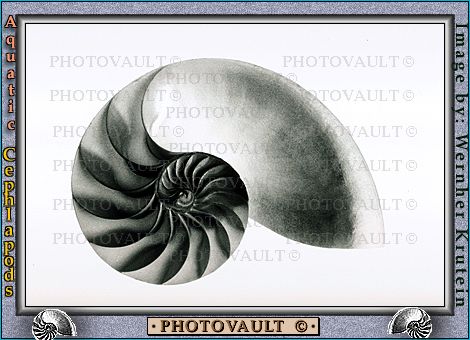
The Nautilus

The first diagram is of the outside of a nautilus shell. The second diagram shows that a spiral can be drawn by putting together quarter circles, one in each new square. This is the golden spiral.  This is present because the growth of the nautilus is proportional to the size of the organism.  A similar curve to this occurs in the shape of a nautilus shell.  The Fibonacci rectangles spiral increases in size by a factor of Phi (1.618..) in a quarter of a turn, the nautilus spiral curve takes a whole turn before points move a factor of 1.618... from the center.  The third diagram is a cross section of a nautilus shell, in which the golden spiral can be seen.   This pattern is also known as the Logarithmic Spiral.

The Human Embryo

As the human embryo develops, it slowly unfolds itself in a pattern similar to the way the golden spiral unfolds itself as it spins farther and farther away from its center.   This pattern is present because the growth of the organism is proportional to the size of the organism   This pattern is also known as the Logarithmic Spiral.

Logarithmic Spirals

    The spiral shapes of a nautilus are called Equiangular or Logarithmic spirals.  If P is any point on the spiral then the length of the spiral from P to the origin is finite. In fact, from the point P which is at distance d from the origin measured along a radius vector, the distance from P to the pole is d sec a.

    The Fibonacci sequence relates closely to the golden ratio and to logarithmic spirals. Logarithmic spirals are simply spirals that increase at a logarithmic rate. The golden ratio, however, is a special fraction equivalent to about 0.618.  A logarithmic spiral can be generated by subdividing a golden rectangle into increasingly smaller squares and golden rectangles. This subdivision begins by fitting a square within the golden rectangle. The remaining space forms a new, smaller golden rectangle. By repeating this process, the spiral form soon becomes evident. Furthermore, the subdivided sections can be thought about as Fibonacci numbers.

    One reason why the logarithmic spiral appears in nature is that it is the result of very simple growth programs such as:

    Grow 1 unit, bend 1 unit
    Grow 2 units, bend 1 unit
    Grow 3 units, bend 1 unit
    And so on...

    Any process which turns or twists at a constant rate but grows or moves with constant acceleration will generate a single logarithmic spiral.

Formulas

Let alpha be the constant angle.

    Parametric: {E^(t Cot[alpha]) Cos[t], E^(t Cot[alpha]) Sin[t]}
    Cartesian: x^2 + y^2 == E^(ArcTan[y/x] Cot[alpha] )
    Polar: r == E^(theta Cot[alpha])
    Pedal: p == r Sin[alpha]
    Whewell: r == s Cos[alpha]
    Cesaro: rho == s Cot[alpha]

Properties

Pursuit Curve

    Pursuit curves are the trace of an object chasing another. Suppose there are n bugs each at a corner of a n sided regular polygon. Each bug crawls towards its next neighbor with uniform speed. The trace of these bugs are equiangular spirals of (n-2)/n * Pi/2 radians (half the angle of the polygon's corner). The figure on the left shows the trace of four bugs, resulting four equiangular spirals of 45 degree. The figure on the right has six objects forming a chasing chain. Each line is the direction of movement and is tangent to the equiangular spirals so formed.

Catacaustic

    Catacaustic of an equiangular spiral with light source at pole is an equal spiral. Proof: Let O be the
pole of the curve. Let O' be the reflection of O through the normal of a variable point P on the curve.
The locus of O' is then an equal spiral since distance[O,O']/distance[O,P] is constant for any P and
equiangular spiral remain unchanged by scaling. Now the reflected ray PO' is just the tangent of O'.

Evolute

    The evolute of an equiangular spiral is an equal spiral, so is its involute. The left figure shows
osculating circles of the curve and their centers (white dots). The right figure shows the curve's
envelope of normals. The original curve is an 80 degree equiangular spiral.

Radial

    The radial of an equiangular spiral is itself scaled. The figure on the left shows a 70 degree
equiangular spiral and its radial. The figure on the right shows its involute, which is another
equiangular spiral.

Inversion

    The inversion of an equiangular spiral with respect to its pole is an equal spiral.

Pedal

    The pedal of an equiangular spiral with respect to its pole is an equal spiral. In the figure, the lines
from pole to the red dots is perpendicular to the tangents (blue lines). The blue curve is an 60 degree
equiangular spiral. The red dots forms its pedal.

Geometric Sequence

    If any part of the curve is scale up or down, it becomes congruent to other parts of the curve.
Lengths of segments (red lines) cut by equally spaced radii (green lines) is a geometric sequence.
Segments of any radius vector cut by the curve is also a geometric sequence, with a multiplier of
E^(2 Pi Cot[alpha]). In the figure, the dots are points on a 85 degree equiangular spiral.

Go back to the Biology and the Golden Ratio page
Go back to the Golden Ratio page