|
Jochen Hurlebaus, Institute for Biotechnology 2, Research
Centre Jülich, 52425 Jülich, Germany
Join our Team:
Simulating Metabolic Networks in Micro-organisms with Dynamic Structured Mathematical Models
Project Overview 2000 Jochen Hurlebaus
Project Goal: Dynamic mathematical models are developed for simulation of metabolic
networks of micro-organisms with focus on bacteria (Escherichia coli).
The goal is to identify control mechanisms in the complicated metabolic
networks of such micro-organisms and make predictions of the influence
of specific genetic modifications (in silico analysis). As a result, simulations
of dynamic cell behaviour under varying fermentation conditions should
be possible (Figure 1).
Figure 1: State of the art tools are able to simulate intracellular steady-state fluxes. Dynamic response of cells to changing fermentation conditions is still difficult to predict and require advanced mathematical models.
Methods: The project
Model development and formulation is done with a Modelling Tool
Software that was produced during the project. The software allows data-fitting
and simulation with identified parameters including graphical output that
is useful for experimental design and is based on a relational database.
Current Project State: The Modelling Tool Software mentioned above is coded in the script language Tcl/Tk. All relevant information of models is stored in a relational database (MySQL, free software for non-commercial use):
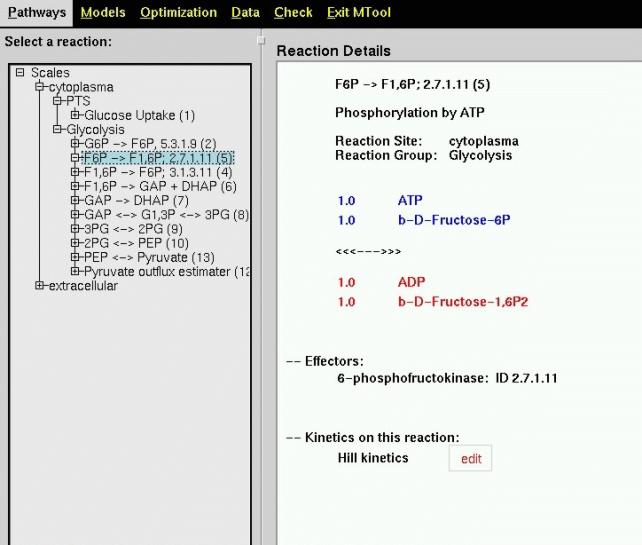
Figure 2 shows presentation of the metabolic network in the Modelling Tool Software: The left part of the image contains a differentiation of the network in different scales set-up by the user (here extracellular and cytoplasm).
Figure 2: Main view of a Metabolic Network in the Modelling
Tool Software. An expandable tree on the left shows the structure, on the
right details of single reactions can be seen.
The Edit button shown next to the Hill Kinetics in Figure 2 leads
to another main feature of the Modelling Tool Software, the detailed definition
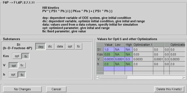
of each kinetic relation. Figure 3 shows the popup window giving the user
full control over the mathematical model.
Figure 3: Control window for set-up of mathematical model details.
The windows main features are:
Complex optimisation - i.e. fitting a high parametric non-linear differential equation model to given data, requires patience and often continued retries. Best results will be retrieved with growing experience on how to set optimisation parameters. This is the reason why the user of the Modelling Tool Software has full control over all optimisation and simulation parameters. After gaining insight in the system with the default values, a user can find parameters that result in the greatest performance for his model and data.
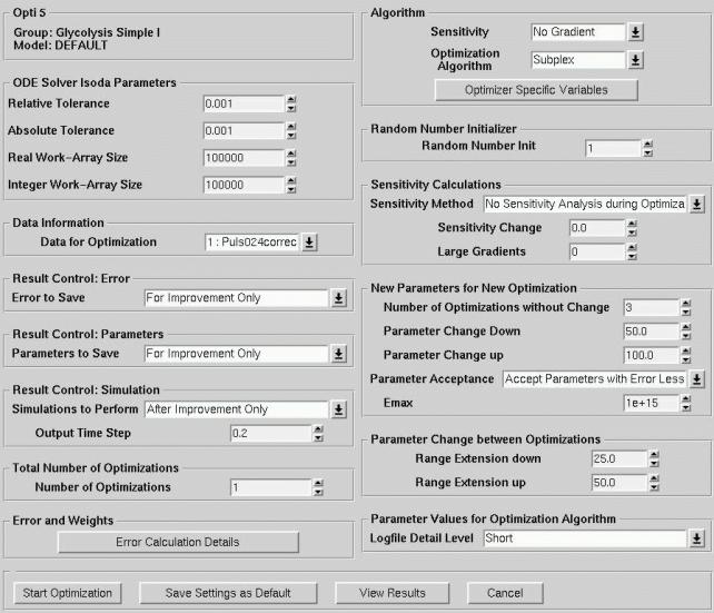
Figure 4: Main Optimisation Window for data-fitting and simulations.
All results, also intermediate results, can be stored and viewed with View
Results
All results of simulations and optimisations are stored automatically.
The user chooses if also intermediate results are stored. Because all details
- including optimisation and simulation parameters, time-steps, used data-file
for fitting, initial parameters and ranges, are stored in the database,
reproduction of all results is possible. Figure 5 shows a window with a
result table of one specific optimisation. The first column shows the sum
of squares of deviations of the model compared with the experimental data.
Double-click on a row displays all details of an simulation or optimisation
respectively. Figure 5 shows an example of the graphical output displaying
amount of metabolite over time.
Graphical output Metabolite concentrations and intracellular fluxes over time calculated and stored can be seen directly on the screen. Often in situations where high-parametric models are fitted without good initial values, graphical output gives good hints on reasons for unsatisfactory performance. A simple least-square-value will not give enough information, therefore graphical output has to be quick and clear. The output of the Modelling Tool Software prints a graph of metabolite concentrations and fluxes over time for each metabolite and flux, including also the experimental data if available for comparison. The Modelling Tool Software can also create Postscript files ready for
printout.
Figure 6: Example of graphical output of metabolite concentrations
over time, produced from parameter fitting to experimental data.
Software Internals The Modelling Tool Software in Tcl/Tk language interacts with
algorithms in Fortran and C for random number generation, solution of the
differential equations, and optimisation. All routines are public-domain
downloaded from the Netlib collection (www.netlib.org). For solution of
the system of differential equations lsoda was chosen because it
works also for stiff equations. The optimisation algorithm used so far
is a modified simplex method. The algorithm was tested on a system of 9
ordinary
differential equations with 47 parameters that was fitted to experimental
data. Data fitting was not successful for all experimental data at the
same time, however, some effects of control could already be identified.
It is therefore thought that the subplex algorithm is useful for optimisation
but the models so far are not. Different algorithms will be tested to answer
the question whether an incorrect model is the reason for the fitting problem.
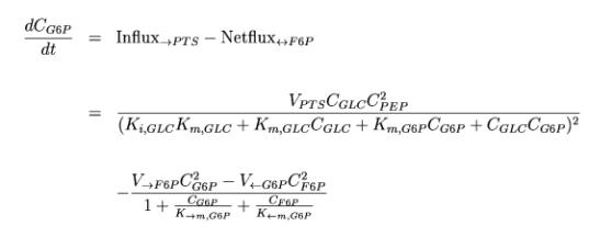
Example: Enzyme Kinetics Two of the 9 differential equations used in the test-model will
be shown here. The first describes the change per time of Glucose-6-Phosphate
in the cell:
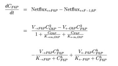
The second kinetic shown here describes the change per time of Fructose-6-Phosphate in the cell:
In principal all reactions of the metabolic network have a similar form
in our model. Changes in the exact mathematical form as well as the amount
of detail of the model can change results significantly. All mathematical
formulations are suggestions and simplifications only. For most cases an
exact formulation cannot be given, in many cases chemical reaction details
are not known.
Good and Bad Examples: I. PTS-System Figure 7 shows results of a model of the PTS-system only. Only
the first peak of the Glucose uptake can be simulated. The reason is that
uptake of Glucose requires Phosphoenolpyruvate which is only available
at the beginning. During the experiment the graphs in Figure 8 show that
the Phosphoenolpyruvate concentration recovered at t=15s resulting in a
new peak of Glucose uptake. But the experiment also shows high Glucose-6-Phosphate
concentrations while Phosphoenolpyruvate is rare at the end of the experiment.
This could not be reproduced with the model that just considered the PTS-uptake
system. A biological explanation, however, is also not available for this
phenomena. We hope to explain this phenomena by including more details
in our model. The above mentioned model with 9 differential equations and
47 parameters was also not able to explain the phenomena. It seems to be
still lacking some control mechanisms of the cell.
Good and Bad Examples: II. Glycolysis System A much more detailed model for the metabolism from Glucose was
developed. It included a complete model for Glycolysis and black-box models
for the Citric-Acid cycle and the Pentose-phosphate pathway. Figure 9 shows
the model components. Two effects of inhibition could be identified that
allow reproduction of the Glucose-6-Phosphate and the Phosphoenolpyruvate
dynamics after the glucose-pulse. The assumptions made are based on experimental
findings from the literature, whereas parameter values are estimated from
literature and with optimisation. Figure 10 shows simulated dynamics of
intracellular Glucose-6-Phosphate and Phosphoenolpyruvate during a pulse
of Glucose.
Sorry we cannot give you all the details about the findings at this
time. Please contact us if you have specific questions.
Figure 10: Simulated intracellular Glucose-6-Phosphate and
Phosphoenolpyruvate concentrations over time during a Glucose-pulse experiment.
The pulse was given at time t=0.
Future prospects: With the availability of the Modelling Tool software now models
can be build and fitted in approximately one hour. The resulting great
development speed for new models has already resulted in a model that describes
dynamic phenomena after a glucose pulse very well. A check of many models
will hopefully provide models that describe all experimental data reasonably.
To choose good models also model selection techniques will be developed.
Additionally, new optimisation algorithms will be tested. In order to identify
shortcomes of current models structure identification would be very helpful.
Some effort will be put in this direction, however, so far no standard
methods are available for structure identification of chemical reaction
networks.
last modified: September 2000
|
||||||||||||||||||||||||||||||||||