INTRODUCTION

Beyond mathematical formulae and analytical solutions, methods utilizing artificial intelligence have not been introduced until recently (Bruines, 1988; Alvarez Grima et al., 2000; Okubo et al., 2003). Nevertheless, they showed very promising results, demonstrating their strong potential in coping with varying issues. In the majority of these research efforts, the main objective is to model the tunneling process and make the performance assessment, based on the experience gained and the data gathered from past projects. However, even though probing risk conditions and identifying vulnerable areas that may disrupt the work progress have been incorporated in the models of many researchers (Einstein et al., 1992; Sinfield and Einstein, 1996), they have not yet been fully addressed, leaving room for further research. These problems are more intense in tunneling projects constructed in complex geological formations (Barla and Pelizza, 2000) and especially in urban areas where the low construction depth and the external loading from the buildings increase risk conditions (Duddeck, 1996; Eisenstein, 1999).

One particular application would be the assessment of Tunnel Boring Machine (TBM) performance which is an important parameter for the successful accomplishment of a tunneling project. With the use and implementation of Artificial Neural Network (ANN), advance rate of tunneling could be modeled with respect to the geological and geotechnical site conditions. This will allow identification and understanding of both the way and the extent that the involved parameters affect the tunneling process. It has been recently presented that generalizations provided by ANN were precise estimations with regards to the anticipated advance rate.

Other applications are also explored and discussed in reference to published papers all throughout the engineering societies around the globe

ARTIFICIAL NEURAL NETWORKS: AN OVERVIEW

 

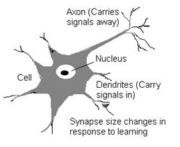
Neurobiological Background

Considered as a neural doctrine, the nervous system of living organisms is a structure consisting of many elements working in parallel and in connection with one another. In 1836, the neuron, the neural cell of the brain, was discovered -- a result worth of the Nobel Prize in 1906. The neuron is a many-inputs-one-output unit. The output can be one of just two possible choices, which is either excited or not excited. The signals from other neurons are summed together and compared against a threshold to determine if the neuron shall be excited. The input signals are subject to attenuation in the synapses which are junction parts of the neuron. The concept of the synapse was introduced in 1897. Figure 1 shows the structure of a neuron.

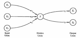
Figure 1 . The structure of neuron (after NIBS Pte Ltd).

 The next important step was to find that the synapse resistance to the incoming signal could be changed during a "learning" process: Hebb's Learning Rule (1949). If an input of a neuron is repeatedly and persistently causing the neuron to fire, a metabolic change happens in the synapse of that particular input to reduce its resistance. This discovery became a basis for the concept of associative memory.

The Artificial Neuron is developed based exactly on the findings previously described, only in mathematical terms. All signals are thought of sending values of 1 or -1 (the "binary" case, often called classic spin). The neuron calculates a weighted sum of inputs and compares it to a threshold. If the sum is higher than the threshold, the output is set to 1, otherwise to -1. The first mathematical representation of the neuron was presented in 1943.

Artificial Neural Networks (ANN)

The power of the neuron comes from its collective behavior in a network where all neurons are interconnected. Their basic characteristic is the ability to perform massively parallel computing of the input stimulus (data), contrary to the customary mathematical models that are based rather on a serial process of mathematical and logical functions (Fausett, 1994). Another advantage of the ANNs is their flexibility in data processing, as no deterministic mathematical relationship of the examined components is required. Instead, once the data is introduced, in a cause�effect mode, the network identifies the existing relationships, learns and mimics their behavior by adjusting the strength of the links between the neurons (connection weights). Thus, they cannot be programmed but they are rather taught through case experience. As a result, soon after the ANN�s training, given an existing dataset, estimates can be drawn for another specific data input. Thus, the trained network can generalize and give estimates for uncertain conditions or even incomplete data (Sietsma and Dow, 1991).

The introduction and analysis of a perceptron (Rosenblat, 1958) led to further understanding of ANN dynamics: a simple neural network consists an input layer, an output layer, and possibly one or more intermediate hidden layers of neurons. Accordingly, each neuron is linked to its neighbors with varying coefficients of connectivity that represent the weighting of these connections. The topology of a simplified ANN is presented in Figure 2. In this simple model, there is one hidden layer having only one neuron. Each neuron of the hidden layer(s) is interconnected to all others found in the input and output layers. The hidden layers are the most important elements of the network as these are the particular parts where the network learns the interdependencies of the model. This learning procedure is accomplished by adjusting the connection weights, impelling the overall network to generate the matching results. In this manner, changing the connection weights (training) causes the network to learn the solution for a given problem. In the topology of Figure 2, each neuron of the input layer (X₁; X₂; X₃) sends out its weighted signal to the Y neuron found in the hidden layer.

 

Figure 2 . Illustration of an artificial neural network structure (after Fausett, 1994).

The combined input signal in the Y neuron has the following form:  

                                                                                                                                                                (1)

where, x_i is the signal of the ith input neuron, w_i the weighting factor of the ith neuron. The input signal (Y_in) is introduced to the activation function of the Y neuron and signaled to the neurons of the output layer, Z₁ and Z₂ following the general form:

                                                                                                                                                                                                      (2)

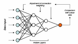
taking into account the weighting of the connection links, namely, v₁ and v₂. This ANN configuration is often called feed-forward.

An observation indicates that the evolving process of an ANN causes it to eventually reach a state where all neurons continue working but no further changes occur. A network may have more than one stable states determined by the choice of synaptic weights and thresholds for the neurons.

There is a training phase when known patterns are presented to the network and its weights are adjusted to produce required outputs. Then, there is a recognition phase when the weights are fixed, the patterns are again presented to the network and it recalls the outputs. A schematic illustration of a feed-forward ANN training is given in Figure 3.

     Figure 3 . Training procedure of a feed-forward ANN with two hidden layers. (after A.G. Benardos , D.C.Kaliampakos)

Weights are adjusted during the training phase and one mostly used is the back-propagation of error method. The initial configuration of ANN is arbitrary; the result of presenting a pattern to the ANN is likely to produce incorrect output. The errors for all input patterns are propagated backwards, from the output layer towards the input layer. The corrections to the weights are selected to minimize the residual error between actual and desired outputs. The algorithm can be viewed as a generalized least squares technique applied to multilayer perceptron. The usual approach of minimizing the errors leads to a system of linear equations; it is important to realize here that its solution is not unique.

The introduction of the concept of an energy function by Hopfield (1982-1986) led to an explosion of work on neural networks. The energy function brought an elegant answer to the problem of ANN convergence to a stable state. In mathematical form, the equation shows a network of N neurons with weights W_ij and output states S_i:

                                                                                                       (3)

The specifics of an evolving ANN allows introduction of this function, which always decreases (or remains unchanged) with each iteration. Evolving of ANNs and even their specifications started to be described in terms of the energy function. Apparently, letting an ANN to evolve eventually shall lead it to a stable state where the energy function has a minimum and cannot change further. The information stored in the synaptic weights W_ij therefore corresponds to some minima of the energy function where the neural network ends up after its evolving process. When the input neurons are clamped to the initial values, the network obtains certain energy in which further evolving will cause it to become more stable in the nearest local minimum.

Another configuration of neural networks is the feedback system. This configuration does not assume propagation of input signal through the hidden layers to the output layers; rather, the output signals of neurons are fed again to the inputs so that evolving continues until stopped externally. The feedback ANN�s are best suited for optimization problems where the neural network looks for the best arrangement of interconnected factors. They are also used for error-correction and partial-contents memories where the stored patterns correspond to the local minima of the energy function.

Optimization problems require a search for the global minimum of the energy function. If we simply let ANN evolve it will reach the nearest local minimum and stop there. To help with the search, one way is to allow for energy fluctuations in ANN by introducing a "probability" that the neuron should fire when the local field is high or should stay calm if the local field is low. In other words, certain amount of chaos is introduced into the ANN evolving process by �shaking". It is important to note that the chaos introduced should be light enough not to shake the system out of the global minimum.

The training sequence of a network is analogous to "shaping" of the energy function, which itself is an optimization problem. The subsequent introduction of the Mean Field Theory proposed by Hopfield (1982) treats neurons as objects with continuous inputs and output states, not just +1 or -1, as in the "classic spin" approach. In the network of neurons, MFT introduces statistical notion of "thermal average", "mean" field V of all input signals of a neuron. To provide the continuity of the neuron outputs, a notion of sigmoid function, g(u), is introduced to be used instead of a simple step-function threshold. The comparison is summarized in Table 1. The widely used sigmoid function is tanh. This approach allows faster stabilization along the energy function

Table 1 . Comparison between the classic spin and mean field theories. (after Ivan Galkin, Univ. Mass Lowell )

  

Limitations of ANN

The critical issue in developing a neural network is this generalization: how well will the network make classification of patterns that are not in the training set?

Applications of neural networks use the ability of ANN to build models of data by capturing the most important features during training period via data fitting. Neural networks, like any other flexible nonlinear estimation methods such as kernel regression and smoothing splines, can suffer from either underfitting or overfitting -- its main disadvantage. An explicit determination of the parameter�s weighting is not an easy task or it may not even be possible in large and complex network architectures (Menhrotra et al., 1997). The reasons behind this are that an ANN operation is based on the following:

�   Data processing occurs in a number of simple processing units (neurons), which have signal inputs and outputs.

�   The neurons� bonding is made through connection links, each one of them having a corresponding weight that multiplies the signal.

      �   Each neuron applies an activation function to the signal input to control the signal output

Moreover, the training set of data may be quite "noisy", which means imprecise. A network that is not sufficiently complex can fail to detect fully the signal in a complicated data set, leading to underfitting. A network that is too complex may fit the noise, not just the signal, leading to overfitting. Overfitting is especially dangerous because it can easily lead to predictions that are far beyond the range of the training data with many of the common types of neural networks. But underfitting can also produce wild predictions in multilayer perceptrons, even with noise-free data.

The best way to avoid overfitting is to use lots of training data. At the same time, the number of weights cannot be arbitrarily reduced for fear of underfitting. Given a fixed amount of training data, there are at least five effective approaches to avoiding underfitting and overfitting, and hence getting good generalization: (1) model selection, (2) jittering, (3) weight decay, (4) early stopping, and (5) Bayesian estimation.

Training a neural network is, in most cases, an exercise in numerical optimization of a usually nonlinear function. There is no single best method for nonlinear optimization; hence, the choice is essentially based on the characteristics of the problem to be solved.

Modeling TBM performance in Athens metro tunnel: A CASE STUDY            (A.G. Benardos, D.C. Kaliampakos, 2000)

The model described here is customized for the construction of an inter-station section of the Athens metro tunnels wherein Tunnel Boring Machines were utilized. Artificial Neural Network (ANN) was used to come up with generalizations with emphasis on the identification of the performance oscillations throughout the tunneling period, capable of providing estimates of the expected tunneling advance rate. The mode, at the same time, was partially used in the identification of difficult ground conditions that may disrupt the work cycle and impair the TBM�s performance.

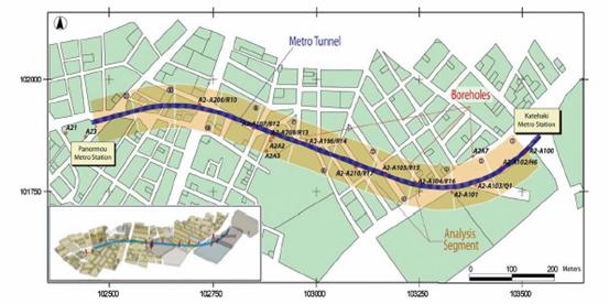
Both outputs, modeling of the TBM�s advance rate and identification of the risk-prone areas, are essential knowledge for the engineers in order to ensure the financial and scheduling credibility of the tunneling project.

Model Synthesis

The model concentrates on the tunnel construction period in soft ground environments. The whole idea follows the ANN philosophy, that is, to analyze the experience gained from the tunnel boring process and to correspond it to a set of selected data. This cause�effect request is used in the ANN so as to identify the interactions between the data and to come up with the exact weighting of the parameters involved, which will finally determine the generalization accuracy. The model�s inputs are based on data relating to the geological and geotechnical characteristics of the subsurface and the specific site conditions. Although machine characteristics (e.g. thrust, torque) are very important for the overall TBM performance, in the case where tunneling is performed in soft rock or complex ground formations, the properties of the ground medium tend to be the most influential ones, as they govern the type and extent of possible failures. Subsequently, encountering ground conditions different from the TBM�s working envelope, affect the achieved tunneling rate (Deere, 1981) and can give rise to claims (Buchi, 1998). Thus, the model considers the geological setting to be the most dominant factor for the TBM performance, as many researchers have also noted (Tarkoy, 1981; Nelson, 1993; Sapigni et al., 2002).

In this way, it is assumed that the characteristics of machine operation remain unchanged and all possible problems and downtime are a direct effect of the geotechnical conditions. Even though downtime is also inflicted by machine failures, logistics support problems, etc., the real question is how the TBM performance is affected by ground conditions and the aforementioned assumption is made exactly so as to be able to evaluate this particular issue. Having that in mind, the data gathering procedure concentrates on obtaining information about the subsurface conditions encountered and the scheduling data, yet excluding all machinery occurred failures (e.g. power failures, belt replacements, etc.).

The selection of the parameters used in the model was made having in mind their capability to credibly represent the ground behavior, hydrogeological environment and site-specific conditions (Benardos, 2002).

These parameters are easily collected in the site-investigation phase and are available to all design stages of the project, without the need for implementing special investigation techniques. More specifically, these parameters are

�   rock mass fracture degree as represented by RQD (P₁),

�   weathering degree of the rock mass (P₂),

�   overload factor�stability factor (N) (P₃),

�   rock mass quality represented by RMR classification (P₄),

�   uniaxial compressive strength of the rock (UCS) (P₅),

�   overburden-construction depth (P₆),

�   hydrogeological conditions represented by the water table surface relative to the tunnel depth (P₇),

�   rock mass permeability (P₈).

Many of them have already been proposed as indicators of the tunneling efficiency. For example, the fracture degree of rock masses is extremely important to TBM tunneling (Deere and Deere, 1988), the overload factor, first introduced by Peck (1969), can provide information about the face stability conditions. In addition, the compressive strength is influencing TBM performance, while RMR is very important as it denotes the tunnel�s stand-up time and is also used in TBM performance analysis (Sapigni et al., 2002). Finally, as Terzaghi (1950) noted the hydrogeological conditions and the presence of water is directly or indirectly linked to the problems occurring in soft ground tunneling.

The study area used for the model development is an interstation tunnel of the Athens Metro. The geological setting is a system of low-level metamorphic sedimentary weak rock consisted of interbedded marly limestones, calcareous sandstones, siltstones, conglomerates, phyllites and schists. The formations are intensely thrusted, folded and faulted with a variable and erratic degree of weathering and alteration (Kavvadas et al., 1996). The examined tunnel is located between the Katehaki and Panormou stations (Figure 4). It is the longest interstation tunnel in the Athens Metro, until now, having a total length of 1129.36m (Attiko Metro SA, 1995a). The examined tunnel length is approximately 1077m, excluding the first 53m (learning curve period). The area is divided in 11 control areas (segments), in which the data is collected and the assessment of the selected geological properties is made (Figure 4). All data from boreholes have been spatially modeled so as to identify the properties especially within the 12m thick stratum that the tunnel is actually being built in, ranging, along the chainage, from the level of +120m to the level of +156m.

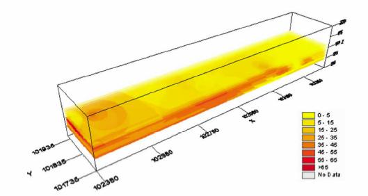
Figure 4. Layout of the examined Athens Metro tunnel (after A.G. Benardos, D.C. Kaliampakos)

For each segment, a corresponding value for every principal parameter is taken. Allocating a representative value for the parameters is accomplished by the spatial modeling of the parameter�s value and by the incorporation of statistical distribution that mimics the parameter�s behavior in each segment (Benardos, 2002). In Figure 5 the spatial modeling of the RQD values is illustrated, for the whole analysis area.

Figure 5. Spatial modeling of the RQD values in the area of the examined tunnel. 

(after A.G. Benardos , D.C. Kaliampakos)

Table 2 . Rating of the principal parameters. (after A.G. Benardos , D.C. Kaliampakos)

 

Table 3 . Expected values of the principal parameters in each segment (after A.G. Benardos , D.C. Kaliampakos)

PARAMETER	Seg1	Seg2	Seg3	Seg4	Seg5	Seg6	Seg7	Seg8	Seg9	Seg10	Seg11
Rock mass fracture degree	0.13	0.88	0.90	0.64	0.72	1.37	1.62	1.26	0.55	0.66	0.74
Rock mass weathering	2.52	2.52	2.24	1.97	1.99	1.89	1.95	1.93	1.96	1.94	1.93
Overload factor	1.07	0.89	1.92	1.99	2.73	2.16	2.49	2.28	2.43	2.61	2.43
Rock mass rating	0.00	0.00	0.36	0.93	1.10	1.83	2.00	1.49	1.08	1.00	1.00
UCS	0.48	0.57	0.97	1.06	1.68	1.31	1.28	1.20	1.16	1.21	1.15
Overburden	0.42	1.00	1.17	1.97	2.86	2.35	1.16	1.45	1.13	0.99	0.88
Water table surface	3.00	2.32	1.71	1.00	0.23	0.02	0.94	1.40	2.17	2.40	2.75
Permeability	1.92	1.97	1.95	1.89	1.86	1.69	1.90	1.82	1.86	1.76	1.81

 

In the next step, the data is categorized in four interval scale classes, from 0 to 3, where 0 denotes the worst case and 3 the best. The limits taken in every class are representative of the specific site conditions and the machine characteristics. In the case of the Athens Metro, the tunnel is constructed in relative low depth and, in general, in weak rock conditions with a double shield TBM machine. The rating of each parameter is presented in Table 2. The limits of the proposed rating transforms the continuous data to a discrete probability structure, a form that is finally used as input to the model. More specifically, the data is introduced to the ANN as the expected values (EV) of the parameters (Table 3). For example, given V₁, V₂, ..., V_n values having a respective probability of occurrence P₁, P₂, ..., P_n, the expected value of the variable X, is estimated as

while,                                                                                                                                               (4)

 

The tunneling advance rate, achieved in each segment, is also introduced into the ANN model. Hence, the input vector of the principal parameters is tallied to the output vector of the mean achieved advance rate, in each segment (Table 4), expressed in m/day (Attiko Metro SA, 1995b). Note that all external origin delays (e.g. strikes, maintenance, etc.) have not been taken into account.

 

Table 4 . Tunneling advance rate data in each of the control segments

(after A.G. Benardos , D.C. Kaliampakos)

   

ANN Development � Feed-forward Configuration

In order to proceed with the development of the ANN model, the dataset � of the whole 11 analysis segments � has been divided into two subsets. The first one (training subset � A) is used for the ANN�s training, whereas the second (test subset � B) is used for the validation of the model�s generalization capability. Special focus is given on the second subset (B), as the network consistency should be ensured for the whole spectrum of cases. Thus, a set incorporating the most representative cases, in terms of the achieved advance rate, has been selected. Apparently, segments no. 2, no. 7 and no. 9, are selected as they represent the worst, the best and an average case. Consequently, the two subsets are comprised by the data collected in the following segments: A={1, 3, 4, 5, 6, 8, 10, 11} and B={2, 7, 9}.

The neural network toolbox of the Matlab software package has been used for building the ANN code and performing the training and testing of the model. The Levenberg�Marquardt algorithm, selected for training the ANNs, is a variation of the classic backpropagation algorithm that, unlike other variations that use heuristics, relies on numerical optimization techniques to minimize and accelerate the required calculations, resulting in much faster training (Demuth and Beale, 1994). More specifically, the direction in which the search is made is described by the following equation:

                                                                                                                                                                                          (5)

where, A_k is the Hessian matrix of the error function at the current values of weights and biases and g_k is the gradient of the error function. Since the error function has the form of a sum of squares the Hessian matrix can be approximated as  and the gradient as  where, J is the Jacobian matrix, which contains first derivatives of the network errors with respect to the weights and biases, and e is a vector of network errors. Finally, the search direction is given by

                                                                                                                                                           (6)

In the case where the scalar l is zero, this is just Newton �s method, using the approximate Hessian matrix. When l is large, this becomes gradient descent with a small step size. Newton �s method is faster and more accurate near an error minimum, so the aim is to shift towards Newton �s method as quickly as possible. Thus, l is decreased after each successful step (reduction in performance function) and is increased only when a tentative step would increase the performance function. In this way, the performance function will always be reduced, at each iteration, of the algorithm.

The ANN�s performance is assessed in terms of the relative error level (D) achieved, between the actual and the predicted advance rate (AR), following the expression:

                                                                                                                                                                               (7)

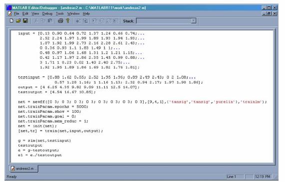
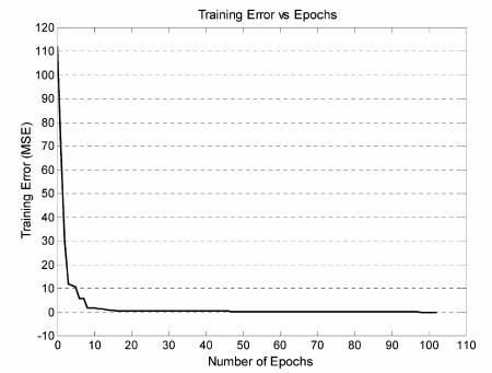
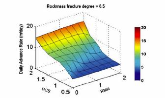
This criterion provides a clear aspect regarding the ANN behavior and moreover makes possible the comparison between the ANN results and other methods or theoretical models focusing on advance rate prediction. A number of test runs have been conducted in order to come up with the network architecture that produces the more consistent results. From the various network architectures that were examined, two particular ANN architectures (8 x 9 x 4 x 1 and 8 x 10 x 7 x 1) proved to be more promising as they responded quite well to the training process. The ANN that was finally selected followed the first architecture, namely the 8 x 9 x 4 x 1 form. This particular structure type means that the ANN has a total of 4 layers, with 8 neurons in the input level, same as the number of the parameters, two hidden layers with 9 and 4 neurons respectively, followed by 1 neuron in the output layer that eventually generates the value of the advance rate. The code used for the ANN development is presented in Figure 6. The mean squared error (MSE) of training for this particular ANN model approximates 1.4x10^-27 and is attained after 103 training epochs, as illustrated in Figure 7. The results generated from the trained model were very satisfactory (Table 5). The relative error between the model outputs and the validation subset ranges in the region of 6% and 8%, reaching a maximum of about 8.4%, a level that is quite acceptable. Furthermore, the ANN behavior shows that the results are consistent in all the validation subset segments, element of major importance for an accurate and effective measurement of the TBM performance. In Figure 8 a surface plot of the model is presented. It has been constructed in relation with the RMR and UCS parameters for a given RQD value of 0.5; the values of all other parameters are taken equal to their mean values. This nomograph can be used as a way of presenting the effect of the selected parameters on the TBM advance rate.

Figure 6. ANN code development in the Matlab Editor/Debugger environment.

(after A.G. Benardos , D.C. Kaliampakos)

Figure 7. Training error vs. training epochs. (after A.G. Benardos , D.C. Kaliampakos)

Figure 8. Surface plot of the expected advance rate with

respect to RMR and UCS for a given RQD value

(after A.G. Benardos , D.C. Kaliampakos)

 

Table 5 . Comparison between the ANN generalization output and the actual advance rate data

(after A.G. Benardos , D.C. Kaliampakos)

 

 

DISCUSSIONS

The field of numerical methods has recently been extended beyond classical plasticity theories to include artificial neural network concepts. In this new approach the numerical simulations can be incorporated as an integral part of the observational method to permit maximum economy and assurance of safety during construction. The results of computations are not more than working hypotheses that have to be subjected to confirmation or modification during construction. In the past, the numerical simulations could not benefit from this type of field observations, but with this new approach, there can be a direct link between precedence and numerical modeling. As construction advances and new field data are obtained the material model can improve as new behavior is observed and learned by the model. Table 6 shows a list of various underground space engineering applications that benefited from the applications artificial neural network.

            Constitutive models based on artificial neural networks are versatile and have the capacity to continuously learn as additional material response data becomes available. These models can capture non-linear material behavior and are increasingly used within various numerical methods for the solution of boundary value problems. Unlike commonly used plasticity models, ANN constitutive models do not require special integration procedures for implementation in FE analysis. The model formulation itself does not use a material stiffness matrix concept in contrast to the elasto-plastic matrix central to conventional plasticity based models.

An empirical method for the design of spans in underground entry-type excavations has been developed based on neural network analysis to an extensive case history database from six Canadian mines. Data were compiled for 292 case histories covering a wide range of rock-mass ratings (RMR) and spans. Rock classification and opening geometry information were part of the input to the analysis and opening stability was the result. The neural network �expert� created by training on the database was used to make predictions on 342 grid points of RMR against span. The span design graph derived from the analysis is shown to be an improvement on existing empirical methods of assessing the stability of underground entry-type excavations  (J. Wang, D. Milne and R. Pakalnis).

            Direct field calibration can take advantage of a rational and systematic approach for incorporating field observations into numerical models. The use of ANN represents a major departure from conventional methods for development and calibration of numerical models using laboratory measurements and field observations whereby such calibration is limited by the capability and complexity of the material constitutive model. It has been demonstrated that the auto-progressive method applied in training of neural network material model from synthetic field data has the capability of extracting relevant material behavior from a series of dual finite element analyses of the excavation. The imposed measured boundary conditions on a finite element model of the excavation aids in the incremental learning process from field observations (Y.M.A. Hashash, C. Marulanda, J. Ghaboussi, S. Jung).

            In the area of deep urban excavations, numerical simulation of construction staging is commonly used to estimate induced ground deformations. A neural network based constitutive model of the soil, given the lateral wall deformation and surface settlement profile measurements, can be generated.  The resulting soil model, used in a numerical analysis, provides correct ground deformations and can be used in the forward prediction of future excavations or later excavation stages. The primary advantage of such model: it can continuously evolve using additional field information.

Artificial neural network is used to adjusts the speed of the shield jack and the speed of the screw conveyor in a shield tunneling (pressure balanced) project in Taipei � a method that proved to be very effective as a means of controlling the shield in various start states. The basic structure of the control system has a learning function based on a back-propagation neural network to model the mechanism of the soil pressure in the soil room of the shield. The learning function renews the model in accordance with the historical records of shield operation. The control mechanism of this system has a searching function to find the optimal value of the desired speed of the shield jack and the screw conveyor to reach the desired soil pressure.

 Table 6. List of various application of ANN in underground excavations and tunneling.

 

CONCLUSIONS

The development of artificial intelligence methods for modeling TBM performance has been well accepted through the scientific community, as the various attempts made in that field proved their efficiency. The ANN systems used in the case study presented and various engineering applications demonstrated satisfactory results in predicting the achieved results. The resulting remarks according to A.G. Benardos and D.C. Kaliampakos on TBM performance modeling:

�   Once trained, the ANN can become a practical off-the-self tool for the prediction of the tunneling advance rate. Its ease of use and its straightforwardness in giving the results can allow its utilization even for on-site assessments.

�   The open source code increases the model�s flexibility, allowing also the insertion of additional data enhancing the prediction accuracy of the final results, even on daily basis.

�   The prediction of the TBM advance rate can be used for the identification of risk-prone areas. As the model is based on geotechnical data, a drop in the advance rate indicates that the area in question may eventually pose threats to the tunneling process and special attention should be paid.

�   The ANN model can also be utilized for a project�s strategic development. Thus, it can be used either for choosing the best tunnel alignment from a number of alternatives, or selecting the most appropriate ground improvement technique if needed to overcome any difficulties or major downtime due to adverse ground conditions. In both cases, scenario analysis can be performed by changing the values of the input parameters, with respect to the proposed tunnel alignment or technique followed. Thus, a direct comparison can be made in financial terms, regarding the best possible selection that would ensure the project�s success.

Through training, neural networks can learn to approximate the relationship between input and output. This process is often explained as a function mapping, that is, training is a procedure to develop a function, embedded in the connection weights, that can describe the relationship between the specified input and output. The power of neural networks function mapping is that it can continuously adapt to new input and output. Once the neural network is trained, it can be used just as a conventional function. Neural network training procedure can be thought of as equivalent to determining a conventional function that involves three major steps: (a) observing the given data, (b) choosing approximate function and (c) calibrating parameters of the function in conventional mapping function creation. Accordingly, neural networks are suitable for a case in which creation of conventional function is difficult, either because of complexity of the given data, or because of continual updating of the data.

Generally, artificial neural network prediction models in deep excavation and tunneling assess the safety of underground structures during construction. Due to the historical information that is gathered during excavations, the limitation of understanding cause and effect, which in turn determines the behavior of the obstacles being modeled, is avoided � a clear advantage of the ANN prediction model.

Finally, it should be noted that in all cases a number of records should be available in order to come up with consistent results. Thus, any model can find its optimal use in cases of intense urban underground development (e.g. subways, sewage tunnels, etc.) as the operations are taking place in roughly the same geological setting, with the same methods and tools, extensive data is available from past projects and a constant data flow can be expected from the worksites.

REFERENCES

 

1.        Alvarez Grima, M., Bruines, P.A., Verhoef, P.N.W, 2000. Modeling tunnel boring machine performance by Neuro-Fuzzy methods. Tunnelling and Underground Space Technology 15 (3), 259�269.

2.        Barton, N.R., 2000. TBM tunnelling in jointed and faulted rock, Balkema.

3.        Benardos, A.G. and Kaliampakos , D.C. , Modelling TBM performance with artificial neural networks, Tunnelling and Underground Space Technology 19 (2004) 597�605.

4.        Bruland, A., 1999. Prediction model for performance and costs. Norwegian TBM Tunnelling, Norwegian Tunnelling Society, pp. 29�34.

5.        Demuth, H., Beale, M., 1994. Neural Network Toolbox User�s Guide. The Mathworks Inc.

6.        Fausett, L., 1994. Fundamentals of Neural Networks. Architectures, Algorithms and Applications. Prentice Hall International Editions, New York .

7.        Galkin, Ivan, Crash Introduction to Artificial Neural Networks, Materials for UML 91.531 Data Mining course, U. MASS Lowell.

8.        Ghaboussi J, Garret JH, Wu X. Knowledge-based modeling of material behaviour with neural networks. Journal of Engineering Mechanics Division (ASCE) 1991; 117(1):132�153.

9.        Ghaboussi J, Pecknold DA, Zhang M, Haj-Ali R. Autoprogressive training of neural network constitutive models. International Journal for Numerical Methods in Engineering 1998; 42(1):105�126.

10.    Ghaboussi J, Sidarta D. A new nested adaptive neural network for modeling of constitutive behaviour of materials. Computers and Geotechnics 1998; 22(1): 29�52.

11.    Ghaboussi J, Sidarta DE . New method of material modeling using neural networks. Proceedings of the 6^th International Symposium on Numerical Models in Geomechanics, 1997; 393�400.

12.    Hashash YMA, Ghaboussi J, Jung S, Marulanda C. Systematic update of a numerical model of a deep excavation using field performance data. Proceedings of the 8th International Symposium on Numerical Models in Geomechanics�NUMOG VIII. Balkema , Italy , 2002; 517�522.

13.    McFeat-Smith, I. , Tarkoy, P.J., 1979. Assessment of tunnel boring performance. Tunnels and Tunnelling, 33�37.

14.    Menhrotra, K., Mohan, C.K., Ranka, S., 1997. Elements of Artificial Neural Networks. MIT Press, Cambridge , MA .

15.    Okubo, S., Kfukui, K., Chen, W., 2003. Expert system for applicability of tunnel boring machines in Japan . Rock Mechanics and Rock Engineering 36 (4), 305�322.

16.    Pande GN, Shin HS. Finite elements with artificial intelligence. Proceedings of the 8th InternationalSymposium on Numerical Models in Geomechanics�NUMOG VIII. Balkema , Italy , 2002; 241�246.

17.    Peck, R., 1969. State of the art report: deep excavations and tunneling in soft ground. In: Proceedings of the Seventh International Conference on Soil Mechanics and Foundation Engineering , Mexico City, pp. 225�290.

18.    Shang, J. Q., Ding, W. and Rowe, R. K. Soil and Rock Characterization Using Complex Permittivity And Artificial Neural Networks, Japanese Geotechnical Journal (October 2004) Vol.44 No.5, pp 15-26.

19.    Shin HS, Pande GN. Enhancement of data for training neural network based constitutive models for geomaterials. Proceedings of the 8th International Symposium on Numerical Models in Geomechanics� NUMOG VIII. Balkema: Italy , 2002; 141�146.

20.    Sietsma, J., Dow, J.F., 1991. Creating artificial neural networks that generalize. Neural Networks (4), 67�79.

21.    Sinfield, J.V., Einstein, H.H., 1996. Evaluation of tunnelling technology using the decision aids in tunnelling. Tunnelling and Underground Space Technology 11 (4), 491�504.

22.    Yeh I.-C., February 1997, Application of neural networks to automatic soil pressure balance control for shield tunneling, Automation in Construction(Elsevier Science), vol. 5, no. 5, pp. 421-426(6).